Inferences About the Difference Between Two Population Means: σ1 and σ2 Known

Letting μ₁ denote the mean of population 1 and μ₂ denote the mean of population 2, we will focus on inferences about the difference between the means: μ₁ – μ₂. To make an inference about this difference, we select a simple random sample of n₁ units from popula­tion 1 and a second simple random sample of n₂ units from population 2. The two samples, taken separately and independently, are referred to as independent simple random samples.

In this section, we assume that information is available such that the two population stan­dard deviations, σ₁ and σ₂, can be assumed known prior to collecting the samples. We refer to this situation as the σ₁ and σ₂ known case. In the following example we show how to compute a margin of error and develop an interval estimate of the difference between the two population means when σ₁ and σ₂ are known.

1. Interval Estimation of  μ1 – μ2

Greystone Department Stores, Inc., operates two stores in Buffalo, New York: One is in the inner city and the other is in a suburban shopping center. The regional manager noticed that products that sell well in one store do not always sell well in the other. The manager believes this situation may be attributable to differences in customer demographics at the two locations. Customers may differ in age, education, income, and so on. Suppose the manager asks us to investigate the difference between the mean ages of the customers who shop at the two stores.

Let us define population 1 as all customers who shop at the inner-city store and popula­tion 2 as all customers who shop at the suburban store.

The difference between the two population means is μ₁ – μ₂.

To estimate μ₁ – μ₂, we will select a simple random sample of n₁ customers from popu­lation 1 and a simple random sample of n₂ customers from population 2. We then compute the two sample means.

x₁ = sample mean age for the simple random sample of n₁ inner-city customers

x₂ = sample mean age for the simple random sample of n₂ suburban customers

The point estimator of the difference between the two population means is the difference between the two sample means.

Figure 10.1 provides an overview of the process used to estimate the difference between two population means based on two independent simple random samples.

 

As with other point estimators, the point estimator x_i — x₂ has a standard error that describes the variation in the sampling distribution of the estimator. With two independent simple random samples, the standard error of x_i— x₂ is as follows:

If both populations have a normal distribution, or if the sample sizes are large enough that the central limit theorem enables us to conclude that the sampling distributions of x_i and x₂ can be approximated by a normal distribution, the sampling distribution of x_i — x₂ will have a normal distribution with mean given by μ₂ — μ₂.

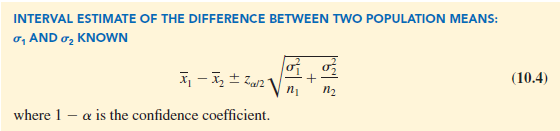
In general, an interval estimate is given by a point estimate ± a margin of error. In the case of estimation of the difference between two population means, an interval estimate will take the following form:

With the sampling distribution of x_i — x₂ having a normal distribution, we can write the margin of error as follows:

Thus the interval estimate of the difference between two population means is as follows:

Let us return to the Greystone example. Based on data from previous customer demo­graphic studies, the two population standard deviations are known with σ₁ = 9 years and s₂ = 10 years. The data collected from the two independent simple random samples of Greystone customers provided the following results.

Using expression (10.1), we find that the point estimate of the difference between the mean ages of the two populations is X₁ – X₂ = 40 – 35 = 5 years. Thus, we estimate that the customers at the inner-city store have a mean age five years greater than the mean age of the suburban store customers. We can now use expression (10.4) to compute the margin of error and provide the interval estimate of Thus the interval estimate of the difference between two population means is as follows: μ₁ – μ₂. Using 95% confidence and z_a/2 = z.₀₂₅ = 1.96, we have

Thus, the margin of error is 4.06 years and the 95% confidence interval estimate of the difference between the two population means is 5 – 4.06 = .94 years to 5 + 4.06 = 9.06 years.

2. Hypothesis Tests About μ₂– μ₂

Let us consider hypothesis tests about the difference between two population means. Using D₀ to denote the hypothesized difference between μ₁ and μ₂, the three forms for a hypothesis test are as follows:

In many applications, D₀ = 0. Using the two-tailed test as an example, when D₀ = 0 the null hypothesis is H₀: μ₁ – m₂ = 0. In this case, the null hypothesis is that m₁ and m₂ are equal. Rejection of H₀ leads to the conclusion that H_a: μ₁ – μ₂ # 0 is true; that is, μ₁ and μ₂ are not equal.

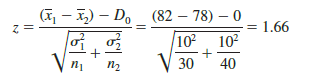
The general steps for conducting hypothesis tests are still applicable here. We must choose a level of significance, compute the value of the test statistic, and find the p-value to determine whether the null hypothesis should be rejected. With two independent simple ran­dom samples, we showed that the point estimator X₁ – X₂ has a standard error s_{Xi 2}– given by expression (10.2) and, when the sample sizes are large enough, the distribution of X₁ – X₂ can be described by a normal distribution. In this case, the test statistic for the difference between two population means when σ₁ and σ₂ are known is as follows.

 

Let us demonstrate the use of this test statistic in the following hypothesis testing example.

As part of a study to evaluate differences in education quality between two training centers, a standardized examination is given to individuals who are trained at the centers. The difference between the mean examination scores is used to assess quality differences between the centers. The population means for the two centers are as follows.

We begin with the tentative assumption that no difference exists between the training quality provided at the two centers. Hence, in terms of the mean examination scores, the null hypothesis is that μ_i – μ₂ = 0. If sample evidence leads to the rejec­tion of this hypothesis, we will conclude that the mean examination scores differ for the two populations. This conclusion indicates a quality differential between the two centers and suggests that a follow-up study investigating the reason for the differen­tial may be warranted. The null and alternative hypotheses for this two-tailed test are written as follows.

The standardized examination given previously in a variety of settings always resulted in an examination score standard deviation near 10 points. Thus, we will use this information to assume that the population standard deviations are known with σ₁ = 10 and σ₂ = 10. An a = .05 level of significance is specified for the study.

Independent simple random samples of n₁ = 30 individuals from training center A and n₂ = 40 individuals from training center B are taken. The respective sample means are x₁ = 82 and x₂ = 78. Do these data suggest a significant difference between the popula­tion means at the two training centers? To help answer this question, we compute the test statistic using equation (10.5).

Next let us compute the p-value for this two-tailed test. Because the test statistic z is in the upper tail, we first compute the area under the curve to the right of z = 1.66. Using the standard normal distribution table, the area to the left of z = 1.66 is .9515. Thus, the area in the upper tail of the distribution is 1.0000 – .9515 = .0485. Because this test is a two­tailed test, we must double the tail area: p-value = 2(.0485) = .0970. Following the usual rule to reject H₀ if p-value < a, we see that the p-value of .0970 does not allow us to reject H₀ at the .05 level of significance. The sample results do not provide sufficient evidence to conclude the training centers differ in quality.

In this chapter we will use the p-value approach to hypothesis testing. However, if you prefer, the test statistic and the critical value rejection rule may be used. With a = .05 and z_a/2 = z.₀₂₅ = 1 96, the rejection rule employing the critical value approach would be reject H₀ if z ≤ -1.96 or if z ≥ 1.96. With z = 1.66, we reach the same do not reject H₀ conclusion.

In the preceding example, we demonstrated a two-tailed hypothesis test about the differ­ence between two population means. Lower tail and upper tail tests can also be considered. These tests use the same test statistic as given in equation (10.5). The procedure for com­puting the p-value and the rejection rules for these one-tailed tests are the same as those for hypothesis tests involving a single population mean and single population proportion.

3. Practical Advice

In most applications of the interval estimation and hypothesis testing procedures presented in this section, random samples with n₁ ≥ 30 and n₂ ≥ 30 are adequate. In cases where either or both sample sizes are less than 30, the distributions of the populations become important considerations. In general, with smaller sample sizes, it is more important for the analyst to be satisfied that it is reasonable to assume that the distributions of the two populations are at least approximately normal.

Source:  Anderson David R., Sweeney Dennis J., Williams Thomas A. (2019), Statistics for Business & Economics, Cengage Learning; 14th edition.