In Chapter 14 we pointed out that standardized residuals are frequently used in residual plots and in the identification of outliers. The general formula for the standardized residual for observation i follows.

The general formula for the standard deviation of residual i is defined as follows.
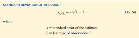
As we stated in Chapter 14, the leverage of an observation is determined by how far the values of the independent variables are from their means. The computation of hp sy _y, and hence the standardized residual for observation i in multiple regression analysis is too complex to be done by hand. However, the standardized residuals can be easily obtained as part of the output from statistical software. Table 15.7 lists the predicted values, the residuals, and the standardized residuals for the Butler Trucking example presented previously in this chapter; we obtained these values by using statistical software. The predicted values in the table are based on the estimated regression equation y = -.869 + .06113x1 + .923x2.
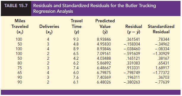
The standardized residuals and the predicted values of y from Table 15.7 are used in Figure 15.10, the standardized residual plot for the Butler Trucking multiple regression example. This standardized residual plot does not indicate any unusual abnormalities. Also, all the standardized residuals are between -2 and +2; hence, we have no reason to question the assumption that the error term e is normally distributed. We conclude that the model assumptions are reasonable.
A normal probability plot also can be used to determine whether the distribution of e appears to be normal. The procedure and interpretation for a normal probability plot were discussed in Section 14.8. The same procedure is appropriate for multiple regression. Again, we would use a statistical software package to perform the computations and provide the normal probability plot.

1. Detecting Outliers
An outlier is an observation that is unusual in comparison with the other data; in other words, an outlier does not fit the pattern of the other data. In Chapter 14 we showed an example of an outlier and discussed how standardized residuals can be used to detect outliers. An observation is classified as an outlier if the value of its standardized residual is less than -2 or greater than +2. Applying this rule to the standardized residuals for the Butler Trucking example (see Table 15.7), we do not detect any outliers in the data set.
In general, the presence of one or more outliers in a data set tends to increase 5, the standard error of the estimate, and hence increase syi-y^i, the standard deviation of residual i. Because syi-y^i appears in the denominator of the formula for the standardized residual (15.23), the size of the standardized residual will decrease as 5 increases. As a result, even though a residual may be unusually large, the large denominator in expression (15.23) may cause the standardized residual rule to fail to identify the observation as being an outlier. We can circumvent this difficulty by using a form of the standardized residuals called studentized deleted residuals.
2. Studentized Deleted Residuals and Outliers
Suppose the ith observation is deleted from the data set and a new estimated regression equation is developed with the remaining n – 1 observations. Let s& denote the standard error of the estimate based on the data set with the ith observation deleted. If we compute the standard deviation of residual i using s& instead of 5, and then compute the standardized residual for observation i using the revised syi-y^i value, the resulting standardized residual is called a studentized deleted residual. If the ith observation is an outlier, 5(i) will be less than 5. The absolute value of the ith studentized deleted residual therefore will be larger than the absolute value of the standardized residual. In this sense, studentized deleted residuals may detect outliers that standardized residuals do not detect.
Many statistical software packages provide an option for obtaining studentized deleted residuals. Using statistical software, we obtained the studentized deleted residuals for the Butler Trucking example; the results are reported in Table 15.8. The t distribution can be used to determine whether the studentized deleted residuals indicate the presence of outliers. Recall that p denotes the number of independent variables and n denotes the number of observations. Hence, if we delete the ith observation, the number of observations in the reduced data set is n – 1; in this case the error sum of squares has (n – 1) – p – 1 degrees of freedom. For the Butler Trucking example with n = 10 and p = 2, the degrees of freedom for the error sum of squares with the ith observation deleted is 9 – 2 – 1 = 6. At a .05 level of significance, the t distribution (Table 2 of Appendix B) shows that with six degrees of freedom, t025 = 2.447. If the value of the ith studentized deleted residual is less than -2.447 or greater than +2.447, we can conclude that the ith observation is an outlier. The studentized deleted residuals in Table 15.8 do not exceed those limits; therefore, we conclude that outliers are not present in the data set.

3. Influential Observations
In Section 14.9 we discussed how the leverage of an observation can be used to identify observations for which the value of the independent variable may have a strong influence on the regression results. As we indicated in the discussion of standardized residuals, the leverage of an observation, denoted hi, measures how far the values of the independent variables are from their mean values. We use the rule of thumb hi > 3(p + 1)/n to identify influential observations. For the Butler Trucking example with p = 2 independent variables and n = 10 observations, the critical value for leverage is 3(2 + 1)/10 = .9. The leverage values for the Butler Trucking example obtained by using statistical software are reported in Table 15.9. Because hi does not exceed .9, we do not detect influential observations in the data set.
4. Using Cook’s Distance Measure to Identify Influential Observations
A problem that can arise in using leverage to identify influential observations is that an observation can be identified as having high leverage and not necessarily be influential in terms of the resulting estimated regression equation. For example, Table 15.10 is a data set consisting of eight observations and their corresponding leverage values (obtained by using statistical software). Because the leverage for the eighth observation is .91 > .75 (the critical leverage value), this observation is identified as influential. Before reaching any final conclusions, however, let us consider the situation from a different perspective.
Figure 15.11 shows the scatter diagram corresponding to the data set in Table 15.10. We used statistical software to develop the following estimated regression equation for these data.
![]()
The straight line in Figure 15.11 is the graph of this equation. Now, let us delete the observation x = 15, y = 39 from the data set and fit a new estimated regression equation to the remaining seven observations; the new estimated regression equation is
![]()

We note that the y-intercept and slope of the new estimated regression equation are very close to the values obtained using all the data. Although the leverage criterion identified the eighth observation as influential, this observation clearly had little influence on the results obtained. Thus, in some situations using only leverage to identify influential observations can lead to wrong conclusions.
Cook’s distance measure uses both the leverage of observation i, hi, and the residual for observation i, (y – yi), to determine whether the observation is influential.
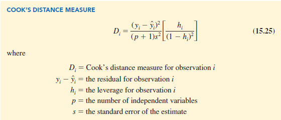
The value of Cook’s distance measure will be large and indicate an influential observation if the residual or the leverage is large. As a rule of thumb, values of Dt > 1 indicate that the ith observation is influential and should be studied further. The last column of Table 15.9 provides Cook’s distance measure for the Butler Trucking problem. Observation 8 with Dt = .650029 has the most influence. However, applying the rule Dt > 1, we should not be concerned about the presence of influential observations in the Butler Trucking data set.
Source: Anderson David R., Sweeney Dennis J., Williams Thomas A. (2019), Statistics for Business & Economics, Cengage Learning; 14th edition.
Great page can’t imagine a more insightful page.