Aggregate Price Indexes

Although price relatives can be used to identify price changes over time for individual items, we are often more interested in the general price change for a group of items taken as a whole. For example, if we want an index that measures the change in the overall cost of living over time, we will want the index to be based on the price changes for a variety of items, including food, housing, clothing, transportation, medical care, and so on. An aggregate price index is developed for the specific purpose of measuring the combined change of a group of items.

Consider the development of an aggregate price index for a group of items categorized as normal automotive operating expenses. For illustration, we limit the items included in the group to gasoline, oil, tire, and insurance expenses.

Table 20.2 gives the data for the four components of our automotive operating expense index for the years 2000 and 2017. With 2000 as the base period, an aggregate price index for the four components will give us a measure of the change in normal automotive operat­ing expenses over the 2000-2017 period.

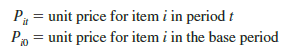
An unweighted aggregate index can be developed by simply summing the unit prices in the year of interest (e.g., 2017) and dividing that sum by the sum of the unit prices in the base year (2000). Let

An unweighted aggregate index for normal automotive operating expenses in t is given by

where the sums are for all items in the group.

An unweighted aggregate index for normal automotive operating expenses in t = 2017 is given by

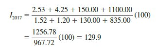
From the unweighted aggregate price index, we might conclude that the price of normal automotive operating expenses has only increased 29.9% over the period from 2000 to 2017. But note that the unweighted aggregate approach to establishing a composite price index for automotive expenses is heavily influenced by the items with large per-unit prices. Conse­quently, items with relatively low unit prices such as gasoline and oil are dominated by the high unit-price items such as tires and insurance. The unweighted aggregate index for auto­motive operating expenses is too heavily influenced by price changes in tires and insurance.

Because of the sensitivity of an unweighted index to one or more high-priced items, this form of aggregate index is not widely used. A weighted aggregate price index provides a better comparison when usage quantities differ.

The philosophy behind the weighted aggregate price index is that each item in the group should be weighted according to its importance. In most cases, the quantity of usage is the best measure of importance. Hence, one must obtain a measure of the quantity of usage for the various items in the group. The fourth column of Table 20.2 gives annual usage information for each item of automotive operating expense based on the typical operation of a midsize automobile for approximately 15,000 miles per year. The quantity weights listed show the expected annual usage for this type of driving situation.

Let Q = quantity of usage for item i. The weighted aggregate price index in period t is given by

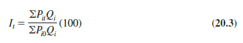
where the sums are for all items in the group. Applied to our automotive operating ex­penses, the weighted aggregate price index is based on dividing total operating costs in 2017 by total operating costs in 2000.

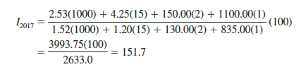
Let t = 2017, and use the quantity weights in Table 20.2. We obtain the following weighted aggregate price index for automotive operating expenses in 2017.

Clearly, compared with the unweighted aggregate index, the weighted index provides a more accurate indication of the price change for automotive operating expenses over the 2000-2017 period. Taking the quantity of usage of gasoline into account helps to offset the smaller percentage increase in insurance costs. The weighted index shows a larger increase in automotive operating expenses than the unweighted index. In general, the weighted aggregate index with quantities of usage as weights is the preferred method for establishing a price index for a group of items.

In the weighted aggregate price index formula (20.3), note that the quantity term Q does not have a second subscript to indicate the time period. The reason is that the quanti­ties Q are considered fixed and do not vary with time as the prices do. The fixed weights or quantities are specified by the designer of the index at levels believed to be representative of typical usage. Once established, they are held constant or fixed for all periods of time the index is in use. Indexes for years other than 2017 require the gathering of new price data P_it, but the weighting quantities Q remain the same.

In a special case of the fixed-weight aggregate index, the quantities are determined from base-year usages. In this case we write Q_t = Q_i0, with the zero subscript indicating base- year quantity weights; formula (20.3) becomes

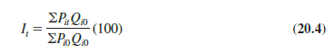
Whenever the fixed quantity weights are determined from base-year usage, the weighted aggregate index is given the name Laspeyres index.

Another option for determining quantity weights is to revise the quantities each period. A quantity Q_it is determined for each year that the index is computed. The weighted aggre­gate index in period t with these quantity weights is given by

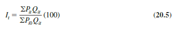
Note that the same quantity weights are used for the base period (period 0) and for period t. However, the weights are based on usage in period t, not the base period. This weighted aggregate index is known as the Paasche index. It has the advantage of being based on current usage patterns. However, this method of computing a weighted aggregate index presents two disadvantages: The normal usage quantities Q_it must be redetermined each year, thus adding to the time and cost of data collection, and each year the index numbers for previous years must be recomputed to reflect the effect of the new quantity weights. Because of these disadvantages, the Laspeyres index is more widely used. The automotive operating expense index was computed with base-period quantities; hence, it is a Laspeyres index. Had usage figures for 2017 been used, it would be a Paasche index. Indeed, because of more fuel efficient cars, gasoline usage decreased and a Paasche index differs from a Laspeyres index.

Source:  Anderson David R., Sweeney Dennis J., Williams Thomas A. (2019), Statistics for Business & Economics, Cengage Learning; 14th edition.