In this section we extend the discussion of inferences about the difference between two population means to the case when the two population standard deviations, s1 and s2, are unknown. In this case, we will use the sample standard deviations, s1 and s2, to estimate the unknown population standard deviations. When we use the sample standard deviations, the interval estimation and hypothesis testing procedures will be based on the t distribution rather than the standard normal distribution.
1. Interval Estimation of μ1 – μ2
In the following example we show how to compute a margin of error and develop an interval estimate of the difference between two population means when s1 and s2 are unknown. Clearwater National Bank is conducting a study designed to identify differences between checking account practices by customers at two of its branch banks. A simple random sample of 28 checking accounts is selected from the Cherry Grove Branch and an independent simple random sample of 22 checking accounts is selected from the Beech- mont Branch. The current checking account balance is recorded for each of the checking accounts. A summary of the account balances follows:

Clearwater National Bank would like to estimate the difference between the mean checking account balance maintained by the population of Cherry Grove customers and the population of Beechmont customers. Let us develop the margin of error and an interval estimate of the difference between these two population means.
In Section 10.1, we provided the following interval estimate for the case when the population standard deviations, s1 and s2, are known.

With σ1 and σ2 unknown, we will use the sample standard deviations σ1 and σ2 to estimate s1 and s2 and replace za/2 with ta/2. As a result, the interval estimate of the difference between two population means is given by the following expression:

In this expression, the use of the t distribution is an approximation, but it provides excellent results and is relatively easy to use. The only difficulty that we encounter in using expression (10.6) is determining the appropriate degrees of freedom for ta/2. Statistical software packages compute the appropriate degrees of freedom automatically. The formula used is as follows:

Let us return to the Clearwater National Bank example and show how to use expression (10.6) to provide a 95% confidence interval estimate of the difference between the population mean checking account balances at the two branch banks. The sample data show n1 = 28, *1 = $1025, and s1 = $150 for the Cherry Grove branch, and n2 = 22, *2 = $910, and s2 = $125 for the Beechmont branch. The calculation for degrees of freedom for ta/2 is as follows:

We round the noninteger degrees of freedom down to 47 to provide a larger t-value and a more conservative interval estimate. Using the t distribution table with 47 degrees of freedom, we find t025 = 2.012. Using expression (10.6), we develop the 95% confidence interval estimate of the difference between the two population means as follows.

The point estimate of the difference between the population mean checking account balances at the two branches is $115. The margin of error is $78, and the 95% confidence interval estimate of the difference between the two population means is 115 – 78 = $37 to 115 + 78 = $193.
2. Hypothesis Tests About μ1 — μ2
Let us now consider hypothesis tests about the difference between the means of two populations when the population standard deviations s1 and s2 are unknown. Letting D0 denote the hypothesized difference between m1 and m2, Section 10.1 showed that the test statistic used for the case where s1 and s2 are known is as follows.

The test statistic, z, follows the standard normal distribution.
When σ1 and σ2 are unknown, we use s1 as an estimator of σ1 and σ2 as an estimator of σ2. Substituting these sample standard deviations for σ1 and σ2 provides the following test statistic when σ1 and σ2 are unknown.
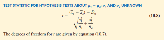
Let us demonstrate the use of this test statistic in the following hypothesis testing example.
Consider a new computer software package developed to help systems analysts reduce the time required to design, develop, and implement an information system. To evaluate the benefits of the new software package, a random sample of 24 systems analysts is selected. Each analyst is given specifications for a hypothetical information system. Then 12 of the analysts are instructed to produce the information system by using current technology. The other 12 analysts are trained in the use of the new software package and then instructed to use it to produce the information system.
This study involves two populations: a population of systems analysts using the current technology and a population of systems analysts using the new software package. In terms of the time required to complete the information system design project, the population means are as follows.

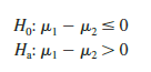
The researcher in charge of the new software evaluation project hopes to show that the new software package will provide a shorter mean project completion time. Thus, the researcher is looking for evidence to conclude that m2 is less than m1; in this case, the difference between the two population means, m1 – m2, will be greater than zero. The research hypothesis m1 – m2 > 0 is stated as the alternative hypothesis. Thus, the hypothesis test becomes
We will use a = .05 as the level of significance.
Suppose that the 24 analysts complete the study with the results shown in Table 10.1. Using the test statistic in equation (10.8), we have

Computing the degrees of freedom using equation (10.7), we have

Rounding down, we will use a t distribution with 21 degrees of freedom. This row of the t distribution table is as follows:

With an upper tail test, the p-value is the area in the upper tail to the right of t = 2.27.
From the above results, we see that the p-value is between .025 and .01. Thus, the p-value is less than a = .05 and H0 is rejected. The sample results enable the researcher to conclude that μ1 − μ2 > 0, or μ1 > μ2. Thus, the research study supports the conclusion that the new software package provides a smaller population mean completion time.
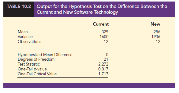
Statistical software can be used to facilitate the testing hypotheses about the difference between two population means. Sample output comparing the current and new software technology is shown in Table 10.2. Table 10.2 displays the test statistic t = 2.27 and its one-tail p-value = .017. Note that statistical software uses equation (10.7) to compute 21 degrees of freedom for
this analysis.
3. Practical Advice
The interval estimation and hypothesis testing procedures presented in this section are robust and can be used with relatively small sample sizes. In most applications, equal or nearly equal sample sizes such that the total sample size n1 + n2 is at least 20 can be expected to provide very good results even if the populations are not normal. Larger sample sizes are recommended if the distributions of the populations are highly skewed or contain outliers. Smaller sample sizes should only be used if the analyst is satisfied that the distributions of the populations are at least approximately normal.
Source: Anderson David R., Sweeney Dennis J., Williams Thomas A. (2019), Statistics for Business & Economics, Cengage Learning; 14th edition.
31 Aug 2021
30 Aug 2021
30 Aug 2021
30 Aug 2021
30 Aug 2021
30 Aug 2021