Kruskal-Wallis Test

In this section we extend the nonparametric procedures to hypothesis tests involving three or more populations. We considered a parametric test for this situation in Chapter 13 when we used quantitative data and assumed that the populations had nor­mal distributions with the same standard deviations. Based on an independent random sample from each population, we used the F distribution to test for differences among the population means.

The nonparametric Kruskal-Wallis test is based on the analysis of independent random samples from each of k populations. This procedure can be used with either ordinal data or quantitative data and does not require the assumption that the populations have normal distributions. The general form of the null and alternative hypotheses is as follows:

H₀: All populations are identical

H_a: Not all populations are identical

If H₀ is rejected, we will conclude that there is a difference among the populations with one or more populations tending to provide smaller or larger values compared to the other populations. We will demonstrate the Kruskal-Wallis test using the following example.

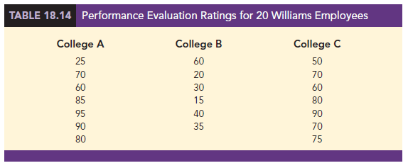
Williams Manufacturing Company hires employees for its management staff from three different colleges. Recently, the company’s personnel director began reviewing the annual performance reports for the management staff in an attempt to determine whether there are differences in the performance ratings among the managers who graduated from the three colleges. Performance rating data are available for independent samples of seven managers who graduated from college A, six managers who graduated from college B, and seven managers who graduated from college C. These data are summarized in Table 18.14. The performance rating shown for each manager is recorded on a scale from 0 to 100, with 100 being the highest possible rating. Suppose we want to test whether the three populations of managers are identical in terms of performance ratings. We will use a .05 level of signific­ance for the test.

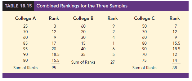
The first step in the Kruskal-Wallis procedure is to rank the combined samples from lowest to highest values. Using all 20 observations in Table 18.14, the lowest rating of 15 for the 4th manager in the college B sample receives a rank of 1. The highest rating of 95 for the 5th manager in the college A sample receives a rank of 20. The performance rating data and their assigned ranks are shown in Table 18.15. Note that we assigned the average ranks to tied performance ratings of 60, 70, 80, and 90. Table 18.15 also shows the sum of ranks for each of the three samples.

The Kruskal-Wallis test statistic uses the sum of the ranks for the three samples and is computed as follows:

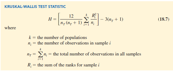
Kruskal and Wallis were able to show that, under the null hypothesis assumption of identical populations, the sampling distribution of H can be approximated by a chi-square distribution with (k – 1) degrees of freedom. This approximation is generally acceptable if the sample sizes for each of the k populations are all greater than or equal to five. The null hypothesis of identical populations will be rejected if the test statistic H is large. As a result, the Kruskal-Wallis test is always expressed as an upper tail test. The computation of the test statistic for the sample data in Table 18.15 is as follows:

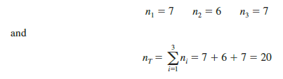
The sample sizes are

Using the sum of ranks for each sample, the value of the Kruskal-Wallis test statistic is as follows:

We can now use the chi-square distribution table (Table 3 of Appendix B) to determ­ine the p–value for the test. Using k – 1 = 3 – 1 = 2 degrees of freedom, we find X² = 7.378 has an area of .025 in the upper tail of the chi-square distribution and x² = 9.21 has an area of .01 in the upper tail of the chi-square distribution. With H = 8.92 between 7.378 and 9.21, we can conclude that the area in the upper tail of the chi-square distribu­tion is between .025 and .01. Because this is an upper tail test, we conclude that the p-value is between .025 and .01. Using JMP or Excel will show the exact p-value for this test. Because p-value < a = .05, we reject H₀ and conclude that the three populations are not all the same. The three populations of performance ratings are not identical and differ signi­ficantly depending upon the college. Because the sum of the ranks is relatively low for the sample of managers who graduated from college B, it would be reasonable for the company to either reduce its recruiting from college B, or at least evaluate the college B graduates more thoroughly before making a hiring decision.

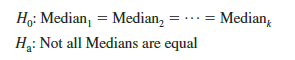
As a final comment, we note that in some applications of the Kruskal-Wallis test, it may be appropriate to make the assumption that the populations have identical shapes and if they differ, it is only by a shift in location for one or more of the populations. If the k populations are assumed to have the same shape, the hypothesis test can be stated in terms of the population medians. In this case, the hypotheses for the Kruskal-Wallis test would be written as follows:

Source:  Anderson David R., Sweeney Dennis J., Williams Thomas A. (2019), Statistics for Business & Economics, Cengage Learning; 14th edition.