Introduction to Monopoly

As the sole producer of a product, a monopolist is in a unique position. If the monopolist decides to raise the price of the product, it need not worry about competitors who, by charging lower prices, would capture a larger share of the market at the monopolist’s expense. The monopolist is the market and com- pletely controls the amount of output offered for sale.

But this does not mean that the monopolist can charge any price it wants—at least not if its objective is to maximize profit. This textbook is a case in point. Pearson Prentice Hall owns the copyright and is therefore a monopoly producer of this book. So why doesn’t it sell the book for $500 a copy? Because few people would buy it, and Prentice Hall would earn a much lower profit.

To maximize profit, the monopolist must first determine its costs and the characteristics of market demand. Knowledge of demand and cost is crucial for a firm’s economic decision making. Given this knowledge, the monopolist must then decide how much to produce and sell. The price per unit that the monopo- list receives then follows directly from the market demand curve. Equivalently, the monopolist can determine price, and the quantity it will sell at that price follows from the market demand curve.

1. Average Revenue and Marginal Revenue

The monopolist’s average revenue—the price it receives per unit sold—is precisely the market demand curve. To choose its profit-maximizing output level, the monopolist also needs to know its marginal revenue: the change in revenue that results from a unit change in output. To see the relationship among total, aver- age, and marginal revenue, consider a firm facing the following demand curve:

P = 6 – Q

Table 10.1 shows the behavior of total, average, and marginal revenue for this demand curve. Note that revenue is zero when the price is $6: At that price, nothing is sold. At a price of $5, however, one unit is sold, so total (and

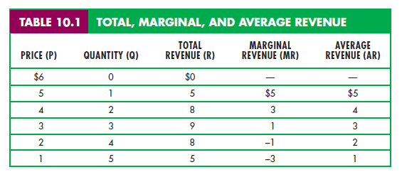
marginal) revenue is $5. An increase in quantity sold from 1 to 2 increases reve- nue from $5 to $8; marginal revenue is thus $3. As quantity sold increases from 2 to 3, marginal revenue falls to $1, and when quantity increases from 3 to 4, mar- ginal revenue becomes negative. When marginal revenue is positive, revenue is increasing with quantity, but when marginal revenue is negative, revenue is decreasing.

When the demand curve is downward sloping, the price (average revenue) is greater than marginal revenue because all units are sold at the same price. If sales are to increase by 1 unit, the price must fall. In that case, all units sold, not just the additional unit, will earn less revenue. Note, for example, what happens in Table 10.1 when output is increased from 1 to 2 units and price is reduced to $4. Marginal revenue is $3: $4 (the revenue from the sale of the additional unit of output) less $1 (the loss of revenue from selling the first unit for $4 instead of $5). Thus, marginal revenue ($3) is less than price ($4).

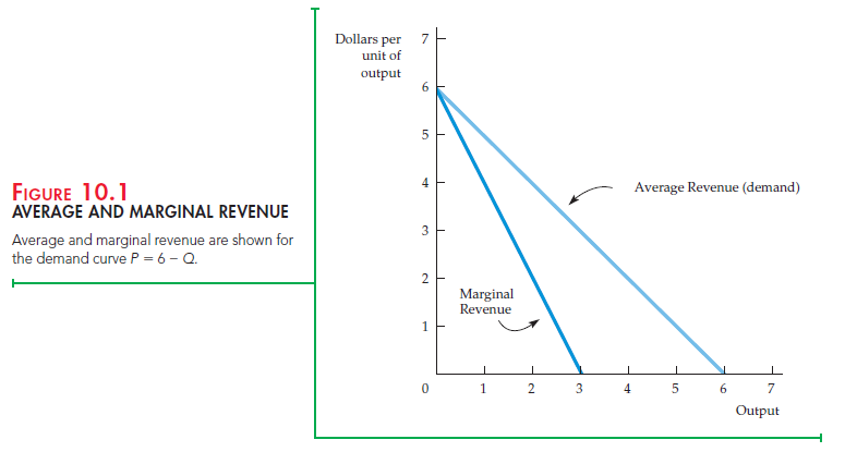
Figure 10.1 plots average and marginal revenue for the data in Table 10.1. Our demand curve is a straight line and, in this case, the marginal revenue curve has twice the slope of the demand curve (and the same intercept).2

2. The Monopolist’s Output Decision

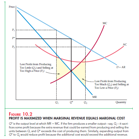
What quantity should the monopolist produce? In Chapter 8, we saw that to maximize profit, a firm must set output so that marginal revenue is equal to marginal cost. This is the solution to the monopolist’s problem. In Figure 10.2, the market demand curve D is the monopolist’s average revenue curve. It speci- fies the price per unit that the monopolist receives as a function of its output level. Also shown are the corresponding marginal revenue curve MR and the average and marginal cost curves, AC and MC. Marginal revenue and marginal cost are equal at quantity Q*. Then from the demand curve, we find the price P* that corresponds to this quantity Q*.

How can we be sure that Q* is the profit-maximizing quantity? Suppose the monopolist produces a smaller quantity Q1 and receives the corresponding higher price P1. As Figure 10.2 shows, marginal revenue would then exceed marginal cost. In that case, if the monopolist produced a little more than Q1,

it would receive extra profit (MR – MC) and thereby increase its total profit. In fact, the monopolist could keep increasing output, adding more to its total profit until output Q*, at which point the incremental profit earned from producing one more unit is zero. So the smaller quantity Q₁ is not profit maxi­mizing, even though it allows the monopolist to charge a higher price. If the monopolist produced Q₁ instead of Q*, its total profit would be smaller by an amount equal to the shaded area below the MR curve and above the MC curve, between Q₁ and Q*.

In Figure 10.2, the larger quantity Q₂ is likewise not profit maximizing. At this quantity, marginal cost exceeds marginal revenue. Therefore, if the monopolist produced a little less than Q₂, it would increase its total profit (by MC – MR). It could increase its profit even more by reducing output all the way to Q*. The increased profit achieved by producing Q* instead of Q₂ is given by the area below the MC curve and above the MR curve, between Q* and Q₂.

We can also see algebraically that Q* maximizes profit. Profit p is the differ­ence between revenue and cost, both of which depend on Q:

As Q is increased from zero, profit will increase until it reaches a maxi­mum and then begin to decrease. Thus the profit-maximizing Q is such that the incremental profit resulting from a small increase in Q is just zero (i.e., Ap / AQ = 0 ).Then

But AR / AQ is marginal revenue and AC / AQ is marginal cost. Thus the profit-maximizing condition is that MR – MC = 0, or MR = MC.

3. An Example

To grasp this result more clearly, let’s look at an example. Suppose the cost of production is

C(Q) = 50 + Q²

In other words, there is a fixed cost of $50, and variable cost is Q². Suppose demand is given by

P(Q) = 40 – Q

By setting marginal revenue equal to marginal cost, you can verify that profit is maximized when Q = 10, an output level that corresponds to a price of $30.

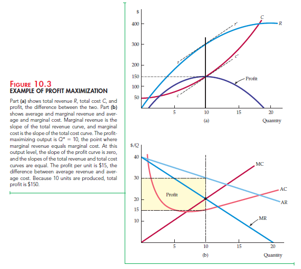
Cost, revenue, and profit are plotted in Figure 10.3(a). When the firm pro­duces little or no output, profit is negative because of the fixed cost. Profit increases as Q increases, reaching a maximum of $150 at Q* = 10, and then decreases as Q is increased further. At the point of maximum profit, the slopes of the revenue and cost curves are the same. (Note that the tangent lines rr’ and cc are parallel.) The slope of the revenue curve is AR/AQ, or marginal revenue, and the slope of the cost curve is AC / AQ, or marginal cost. Because profit is maximized when marginal revenue equals marginal cost, the slopes are equal.

Figure 10.3(b) shows both the corresponding average and marginal revenue curves and average and marginal cost curves. Marginal revenue and marginal cost intersect at Q* = 10. At this quantity, average cost is $15 per unit and price is $30 per unit. Thus average profit is $30 – $15 = $15 per unit. Because 10 units are sold, profit is (10)($15) = $150, the area of the shaded rectangle.

4. A Rule of Thumb for Pricing

We know that price and output should be chosen so that marginal revenue equals marginal cost, but how can the manager of a firm find the correct price and output level in practice? Most managers have only limited knowledge of the average and marginal revenue curves that their firms face. Similarly, they might know the firm’s marginal cost only over a limited output range. We there- fore want to translate the condition that marginal revenue should equal mar- ginal cost into a rule of thumb that can be more easily applied in practice.

To do this, we first write the expression for marginal revenue:

Note that the extra revenue from an incremental unit of quantity, A (PQ)/ AQ, has two

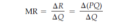
components:

1. Producing one extra unit and selling it at price P brings in revenue (1)(P) = P.
2. But because the firm faces a downward-sloping demand curve, producing and selling this extra unit also results in a small drop in price AP / AQ which reduces the revenue from all units sold (i.e., a change in revenue Q[A P / AQ]).

Thus,

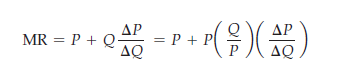
We obtained the expression on the right by taking the term Q(AP/AQ) and The elasticity of demand is multiplying and dividing it by P. Recall that the elasticity of demand is defined ^{discussed in} §§².^{4 and 4}A. as E_d = (P / Q)(AQ / AP). Thus (Q / P)(AP / AQ) is the reciprocal of the elastic­ity of demand, 1/E_d, measured at the profit-maximizing output, and

MR = P + P(1/Ed)

Now, because the firm’s objective is to maximize profit, we can set marginal revenue equal to marginal cost:

P + P(l/Ed) = MC

which can be rearranged to give us

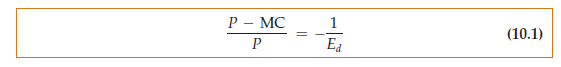
This relationship provides a rule of thumb for pricing. The left-hand side, (P – MC)/P, is the markup over marginal cost as a percentage of price. The relationship says that this markup should equal minus the inverse of the elasticity of demand.4 (This figure will be a positive number because the elasticity of demand is negative.) Equivalently, we can rearrange this equation to express price directly as a markup over marginal cost:

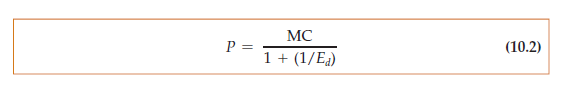
For example, if the elasticity of demand is −4 and marginal cost is $9 per unit, price should be $9/(1  – 1/4)  = $9/.75  = $12 per unit.

How does the price set by a monopolist compare with the price under compe- tition? In Chapter 8, we saw that in a perfectly competitive market, price equals marginal cost. A monopolist charges a price that exceeds marginal cost, but by an amount that depends inversely on the elasticity of demand. As the markup equation (10.1) shows, if demand is extremely elastic, Ed  is a large negative number, and price will be very close to marginal cost. In that case, a monopolized market will

look much like a competitive one. In fact, when demand is very elastic, there is little benefit to being a monopolist.

Also note that a monopolist will never produce a quantity of output that is on the inelastic portion of the demand curve—i.e., where the elasticity of demand is less than 1 in absolute value. To see why, suppose that the monopolist is pro- ducing at a point on the demand curve where the elasticity is −0.5. In that case, the monopolist could make a greater profit by producing less and selling at a higher price. (A 10-percent reduction in output, for example, would allow for a

20-percent increase in price and thus a 10-percent increase in revenue. If marginal cost were greater than zero, the increase in profit would be even more than 10 percent because the lower output would reduce the firm’s costs.) As the monopo- list reduces output and raises price, it will move up the demand curve to a point where the elasticity is greater than 1 in absolute value and the markup rule of equation (10.2) will be satisfied.

Suppose, however, that marginal cost is zero. In that case, we cannot use equation (10.2) directly to determine the profit-maximizing price. However, we can see from equation (10.1) that in order to maximize profit, the firm will pro- duce at the point where the elasticity of demand is exactly −1. If marginal cost is zero, maximizing profit is equivalent to maximizing revenue, and revenue is maximized when Ed   =  – 1.

Source: Pindyck Robert, Rubinfeld Daniel (2012), Microeconomics, Pearson, 8th edition.