Measures of Variability

In addition to measures of location, it is often desirable to consider measures of variability, or dispersion. For example, suppose that you are a purchasing agent for a large manufacturing firm and that you regularly place orders with two different suppliers. After several months of operation, you find that the mean number of days required to fill orders is 10 days for both of the suppliers. The histograms summarizing the number of working days required to fill orders from the suppliers are shown in Figure 3.2. Although the mean number of days is 10 for both suppliers, do the two suppliers demonstrate the same degree of reliability in terms of making deliveries on schedule? Note the dispersion, or variability, in delivery times indicated by the histograms. Which supplier would you prefer?

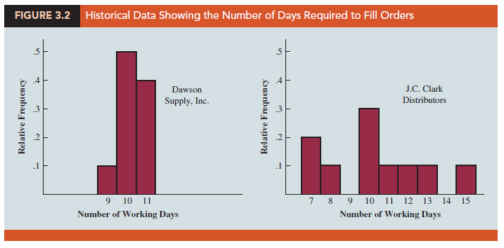
For most firms, receiving materials and supplies on schedule is important. The 7- or 8-day deliveries shown for J.C. Clark Distributors might be viewed favorably; however, a few of the slow 13- to 15-day deliveries could be disastrous in terms of keeping a work­force busy and production on schedule. This example illustrates a situation in which the variability in the delivery times may be an overriding consideration in selecting a supplier. For most purchasing agents, the lower variability shown for Dawson Supply, Inc., would make Dawson the preferred supplier.

We turn now to a discussion of some commonly used measures of variability.

1. Range

The simplest measure of variability is the range.

Let us refer to the data on starting salaries for business school graduates in Table 3.1. The largest starting salary is 6325 and the smallest is 5710. The range is 6325 – 5710 = 615.

Although the range is the easiest of the measures of variability to compute, it is sel­dom used as the only measure. The reason is that the range is based on only two of the observations and thus is highly influenced by extreme values. Suppose the highest paid graduate received a starting salary of $15,000 per month. In this case, the range would be 15,000 – 5710 = 9290 rather than 615. This large value for the range would not be especially descriptive of the variability in the data because 11 of the 12 starting salaries are closely grouped between 5710 and 6130.

2. Interquartile Range

A measure of variability that overcomes the dependency on extreme values is the interquartile range (IQR). This measure of variability is the difference between the third quartile, Q₃, and the first quartile, Q₁. In other words, the interquartile range is the range for the middle 50% of the data.

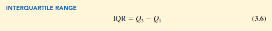
For the data on monthly starting salaries, the quartiles are Q₃ = 6000 and Q₁ = 5865.

Thus, the interquartile range is 6000 – 5865 = 135.

3. Variance

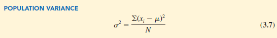
The variance is a measure of variability that utilizes all the data. The variance is based on the difference between the value of each observation (xi) and the mean. The difference between each x_i and the mean (X for a sample, m for a population) is called a deviation about the mean. For a sample, a deviation about the mean is written (x_i – X); for a popu­lation, it is written (x_;. – m). In the computation of the variance, the deviations about the mean are squared.

If the data are for a population, the average of the squared deviations is called the population variance. The population variance is denoted by the Greek symbol s². For a population of N observations and with m denoting the population mean, the definition of the population variance is as follows.

In most statistical applications, the data being analyzed are for a sample. When we compute a sample variance, we are often interested in using it to estimate the population variance s². Although a detailed explanation is beyond the scope of this text, it can be shown that if the sum of the squared deviations about the sample mean is divided by n – 1, and not n, the resulting sample variance provides an unbiased estimate of the population variance. For this reason, the sample variance, denoted by s², is defined as follows.

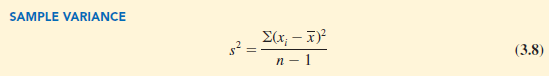
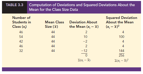
To illustrate the computation of the sample variance, we will use the data on class size for the sample of five college classes as presented in Section 3.1. A summary of the data, including the computation of the deviations about the mean and the squared deviations about the mean, is shown in Table 3.3. The sum of squared deviations about the mean is S(x_i – X )² = 256. Hence, with n – 1 = 4, the sample variance is

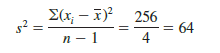
Before moving on, let us note that the units associated with the sample variance often cause confusion. Because the values being summed in the variance calculation, (X – X)², are squared, the units associated with the sample variance are also squared. For instance, the sample variance for the class size data is s² = 64 (students)². The squared units associated with variance make it difficult to develop an intuitive under­standing and interpretation of the numerical value of the variance. We recommend that you think of the variance as a measure useful in comparing the amount of variability for two or more variables. In a comparison of the variables, the one with the largest variance shows the most variability. Further interpretation of the value of the variance may not be necessary.

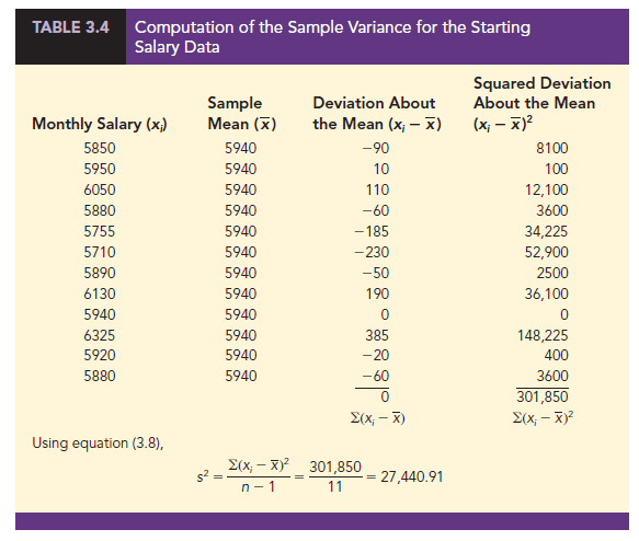
As another illustration of computing a sample variance, consider the starting sala­ries listed in Table 3.1 for the 12 business school graduates. In Section 3.1, we showed that the sample mean starting salary was 5940. The computation of the sample variance (s² = 27,440.91) is shown in Table 3.4.

In Tables 3.3 and 3.4 we show both the sum of the deviations about the mean and the sum of the squared deviations about the mean. For any data set, the sum of the deviations about the mean will always equal zero. Note that in Tables 3.3 and 3.4, S(x_t – X) = 0.

The positive deviations and negative deviations cancel each other, causing the sum of the deviations about the mean to equal zero.

4. Standard Deviation

The standard deviation is defined to be the positive square root of the variance. Following the notation we adopted for a sample variance and a population variance, we use s to de­note the sample standard deviation and s to denote the population standard deviation. The standard deviation is derived from the variance in the following way.

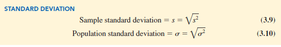
Recall that the sample variance for the sample of class sizes in five college classes is s² = 64. Thus, the sample standard deviation is s = V64 = 8. For the data on starting salaries, the sample standard deviation is s = √27,440.91 = 165.65.

What is gained by converting the variance to its corresponding standard deviation? Recall that the units associated with the variance are squared. For example, the sample variance for the starting salary data of business school graduates is s^{[1] [2] [3]} = 27,440.91 (dol­lars).² Because the standard deviation is the square root of the variance, the units of the variance, dollars squared, are converted to dollars in the standard deviation. Thus, the stan­dard deviation of the starting salary data is $165.65. In other words, the standard deviation is measured in the same units as the original data. For this reason the standard deviation is more easily compared to the mean and other statistics that are measured in the same units as the original data.

5. Coefficient of Variation

In some situations we may be interested in a descriptive statistic that indicates how large the standard deviation is relative to the mean. This measure is called the coefficient of variation and is usually expressed as a percentage.

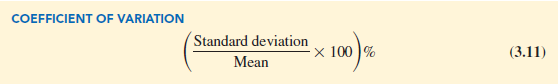
For the class size data, we found a sample mean of 44 and a sample standard deviation of 8. The coefficient of variation is [(8/44) x 100]% = 18.2%. In words, the coefficient of variation tells us that the sample standard deviation is 18.2% of the value of the sam­ple mean. For the starting salary data with a sample mean of 3940 and a sample standard deviation of 165.65, the coefficient of variation, [(165.65/5940) X 100]% = 2.8%, tells us the sample standard deviation is only 2.8% of the value of the sample mean. In general, the coefficient of variation is a useful statistic for comparing the variability of variables that have different standard deviations and different means.

Source:  Anderson David R., Sweeney Dennis J., Williams Thomas A. (2019), Statistics for Business & Economics, Cengage Learning; 14th edition.