Population Mean: σ Known

In order to develop an interval estimate of a population mean, either the population stand­ard deviation s or the sample standard deviation 5 must be used to compute the margin of error. In most applications s is not known, and 5 is used to compute the margin of error. In some applications, large amounts of relevant historical data are available and can be used to estimate the population standard deviation prior to sampling. Also, in quality control applications where a process is assumed to be operating correctly, or “in control,” it is ap­propriate to treat the population standard deviation as known. We refer to such cases as the σ known case. In this section we introduce an example in which it is reasonable to treat s as known and show how to construct an interval estimate for this case.

Each week Lloyd’s Department Store selects a simple random sample of 100 customers in order to learn about the amount spent per shopping trip. With x representing the amount spent per shopping trip, the sample mean x provides a point estimate of μ, the mean amount spent per shopping trip for the population of all Lloyd’s customers. Lloyd’s has been using the weekly survey for several years. Based on the historical data, Lloyd’s now assumes a known value of s = $20 for the population standard deviation. The historical data also indicate that the population follows a normal distribution.

During the most recent week, Lloyd’s surveyed 100 customers (n = 100) and obtained a sample mean of x = $82. The sample mean amount spent provides a point estimate of the population mean amount spent per shopping trip, μ. In the discussion that follows, we show how to compute the margin of error for this estimate and develop an interval estimate of the population mean.

1. Margin of Error and the Interval Estimate

In Chapter 7 we showed that the sampling distribution of x can be used to compute the probability that x will be within a given distance of μ. In the Lloyd’s example, the historical data show that the population of amounts spent is normally distributed with a standard deviation of σ = 20. So, using what we learned in Chapter 7, we can conclude that the sampling distribution of x follows a normal distribution with a standard error of σ_x = σ/√n = 20/√100 = 2. This sampling distribution is shown in Figure 8.I.¹ Because the sampling distribution shows how values of x are distributed around the population mean m, the sampling distribution of x provides information about the possible differences between x and m.

Using the standard normal probability table, we find that 95% of the values of any nor­mally distributed random variable are within ±1.96 standard deviations of the mean. Thus, when the sampling distribution of x is normally distributed, 95% of the x values must be within ± 1.96s_x of the mean m. In the Lloyd’s example we know that the sampling distribu­tion of x is normally distributed with a standard error of σ_x = 2. Because ± 1.96s_x = 1.96(2) = 3.92, we can conclude that 95% of all x values obtained using a sample size of n = 100 will be within ±3.92 of the population mean m. See Figure 8.2.

In the introduction to this chapter we said that the general form of an interval estimate of the population mean m is x ± margin of error. For the Lloyd’s example, suppose we set the margin of error equal to 3.92 and compute the interval estimate of m using x ± 3.92. To provide an interpretation for this interval estimate, let us consider the values of x that could be obtained if we took three different simple random samples, each consisting of 100 Lloyd’s customers. The first sample mean might turn out to have the value shown as X₁ in Figure 8.3. In this case, Figure 8.3 shows that the interval formed by subtracting 3.92 from X₁ and adding 3.92 to X₁ includes the population mean m. Now consider what happens if the second sample mean turns out to have the value shown as X₂ in Figure 8.3.

Although this sample mean differs from the first sample mean, we see that the interval formed by subtracting 3.92 from X₂ and adding 3.92 to X₂ also includes the population mean μ. However, consider what happens if the third sample mean turns out to have the value shown as X₃ in Figure 8.3. In this case, the interval formed by subtracting 3.92 from X₃ and adding 3.92 to X₃ does not include the population mean m. Because X₃ falls in the upper tail of the sampling distribution and is farther than 3.92 from μ, subtracting and adding 3.92 to X₃ forms an interval that does not include μ.

Any sample mean X that is within the darkly shaded region of Figure 8.3 will provide an interval that contains the population mean μ. Because 95% of all possible sample means are in the darkly shaded region, 95% of all intervals formed by subtracting 3.92 from X and adding 3.92 to X will include the population mean μ.

Recall that during the most recent week, the quality assurance team at Lloyd’s surveyed 100 customers and obtained a sample mean amount spent of X = 82. Using X ± 3.92 to construct the interval estimate, we obtain 82 ± 3.92. Thus, the specific interval estimate of μ based on the data from the most recent week is 82 – 3.92 = 78.08 to 82 + 3.92 = 85.92. Because 95% of all the intervals constructed using X ± 3.92 will contain the popu­lation mean, we say that we are 95% confident that the interval 78.08 to 85.92 includes the population mean μ. We say that this interval has been established at the 95% confidence level. The value .95 is referred to as the confidence coefficient, and the interval 78.08 to 85.92 is called the 95% confidence interval.

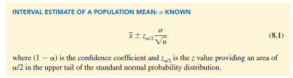
Let us use expression (8.1) to construct a 95% confidence interval for the Lloyd’s example. For a 95% confidence interval, the confidence coefficient is (1 – a) = .95 and thus, a = .05. Using the standard normal probability table, an area of a/2 = .05/2 = .025 in the upper tail provides z.₀₂₅ = 1.96. With the Lloyd’s sample mean X = 82, s = 20, and a sample size n = 100, we obtain

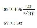
Thus, using expression (8.1), the margin of error is 3.92 and the 95% confidence interval is 82 – 3.92 = 78.08 to 82 + 3.92 = 85.92.

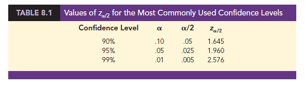
Although a 95% confidence level is frequently used, other confidence levels such as 90% and 99% may be considered. Values of z_a/2 for the most commonly used confidence levels are shown in Table 8.1. Using these values and expression (8.1), the 90% confidence interval for the Lloyd’s example is

Thus, at 90% confidence, the margin of error is 3.29 and the confidence interval is 82 − 3.29 = 78.71 to 82 + 3.29 = 85.29. Similarly, the 99% confidence interval is

Thus, at 99% confidence, the margin of error is 5.15 and the confidence interval is 82 − 5.15 = 76.85 to 82 + 5.15 = 87.15.

Comparing the results for the 90%, 95%, and 99% confidence levels, we see that in order to have a higher degree of confidence, the margin of error and thus the width of the confidence interval must be larger.

2. Practical Advice

If the population follows a normal distribution, the confidence interval provided by ex­pression (8.1) is exact. In other words, if expression (8.1) were used repeatedly to generate 95% confidence intervals, exactly 95% of the intervals generated would contain the popula­tion mean. If the population does not follow a normal distribution, the confidence interval provided by expression (8.1) will be approximate. In this case, the quality of the approxim­ation depends on both the distribution of the population and the sample size.

In most applications, a sample size of n > 30 is adequate when using expression (8.1) to develop an interval estimate of a population mean. If the population is not normally distrib­uted but is roughly symmetric, sample sizes as small as 15 can be expected to provide good approximate confidence intervals. With smaller sample sizes, expression (8.1) should only be used if the analyst believes, or is willing to assume, that the population distribution is at least approximately normal.

Source:  Anderson David R., Sweeney Dennis J., Williams Thomas A. (2019), Statistics for Business & Economics, Cengage Learning; 14th edition.