Multiple Comparison Procedures

When we use analysis of variance to test whether the means of k populations are equal, rejection of the null hypothesis allows us to conclude only that the population means are not all equal. In some cases we will want to go a step further and determine where the differ­ences among means occur. The purpose of this section is to show how multiple comparison procedures can be used to conduct statistical comparisons between pairs of population means.

1. Fisher’s LSD

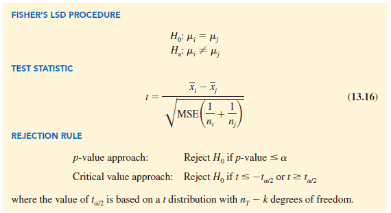
Suppose that analysis of variance provides statistical evidence to reject the null hypothesis of equal population means. In this case, Fisher’s least significant difference (LSD) proced­ure can be used to determine where the differences occur. To illustrate the use of Fisher’s LSD procedure in making pairwise comparisons of population means, recall the Chemitech experiment introduced in Section 13.1. Using analysis of variance, we concluded that the mean number of units produced per week are not the same for the three assembly methods. In this case, the follow-up question is: We believe the assembly methods differ, but where do the differences occur? That is, do the means of populations 1 and 2 differ? Or those of populations 1 and 3? Or those of populations 2 and 3? The following summarizes Fisher’s LSD procedure for comparing pairs of population means.

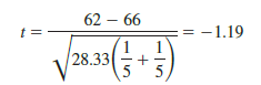
Let us now apply this procedure to determine whether there is a significant difference between the means of population 1 (method A) and population 2 (method B) at the a = .05 level of significance. Table 13.1 showed that the sample mean is 62 for method A and 66 for method B. Table 13.3 showed that the value of MSE is 28.33; it is the estimate of s2 and is based on 12 degrees of freedom. For the Chemitech data the value of the test statistic is

Because we have a two-tailed test, the p-value is two times the area under the curve for the t distribution to the left of t = −1.19. Using Table 2 in Appendix B, the t distribution table for 12 degrees of freedom provides the following information.

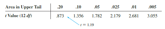
The t distribution table only contains positive t values. Because the t distribution is symmetric, however, we can find the area under the curve to the right of t = 1.19 and double it to find the p-value corresponding to t = −1.19. We see that t = 1.19 is between .20 and .10. Doubling these amounts, we see that the p-value must be between .40 and .20. Statistical software can be used to show that the exact p-value is .2571. Because the p-valueis greater th an a = .05, we cannot reject the null hypothesis. Hence, we cannot concludethat the population mean number of units produced per week for  method A is different from the population mean for method B.

Many practitioners find it easier to determine how large the difference between the sample means must be to reject H0. In this case the test statistic is xi 2 xj, and the test is conducted by the following procedure.

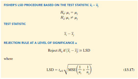
For the Chemitech experiment the value of LSD is

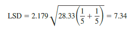
Note that when the sample sizes are equal, only one value for LSD is computed. In such cases we can simply compare the magnitude of the difference between any two sample means with the value of LSD. For example, the difference between the sample means for population 1 (Method A) and population 3 (Method C) is 62 – 52 = 10. This difference is greater than LSD = 7.34, which means we can reject the null hypothesis that the population mean number of units produced per week for Method A is equal to the population mean for Method C. Similarly, with the difference between the sample means for populations 2 and 3 of 66 – 52 = 14 > 7.34, we can also reject the hypothesis that the population mean for Method B is equal to the population mean for Method C. In effect, our conclusion is that the popula­tion means for Method A and Method B both differ from the population mean for Method C.

Fisher’s LSD can also be used to develop a confidence interval estimate of the difference between the means of two populations. The general procedure follows.

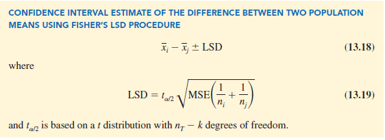
If the confidence interval in expression (13.18) includes the value zero, we cannot reject the hypothesis that the two population means are equal. However, if the confidence interval does not include the value zero, we conclude that there is a difference between the population means. For the Chemitech experiment, recall that LSD = 7.34 (corresponding to t.₀₂₅ = 2.179). Thus, a 95% confidence interval estimate of the difference between the means of populations 1 and 2 is 62 – 66 ± 7.34 = -4 ± 7.34 = -11.34 to 3.34; because this interval includes zero, we cannot reject the hypothesis that the two population means are equal.

2. Type I Error Rates

We began the discussion of Fisher’s LSD procedure with the premise that analysis of vari­ance gave us statistical evidence to reject the null hypothesis of equal population means. We showed how Fisher’s LSD procedure can be used in such cases to determine where the dif­ferences occur. Technically, it is referred to as a protected or restricted LSD test because it is employed only if we first find a significant F value by using analysis of variance. To see why this distinction is important in multiple comparison tests, we need to explain the difference between a comparisonwise Type I error rate and an experimentwise Type I error rate.

In the Chemitech experiment we used Fisher’s LSD procedure to make three pairwise comparisons.

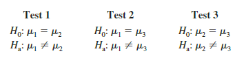
In each case, we used a level of significance of a = .05. Therefore, for each test, if the null hypothesis is true, the probability that we will make a Type I error is a = .05; hence, the probability that we will not make a Type I error on each test is 1 – .05 = .95. In discussing multiple comparison procedures we refer to this probability of a Type I error (a = .05) as the comparisonwise Type I error rate; comparisonwise Type I error rates indicate the level of significance associated with a single pairwise comparison.

Let us now consider a slightly different question. What is the probability that in making three pairwise comparisons, we will commit a Type I error on at least one of the three tests? To answer this question, note that the probability that we will not make a Type I error on any of the three tests is (.95)(.95)(.95) = .8574.^[1] Therefore, the probability of making at least one Type I error is 1 – .8574 = .1426. Thus, when we use Fisher’s LSD procedure to make all three pairwise comparisons, the Type I error rate associated with this approach is not .05, but actually .1426; we refer to this error rate as the overall or experimentwise Type I error rate. To avoid confusion, we denote the experimentwise Type I error rate as a_EW.

The experimentwise Type I error rate gets larger for problems with more populations.

For example, a problem with five populations has 10 possible pairwise comparisons. If we tested all possible pairwise comparisons by using Fisher’s LSD with a comparisonwise error rate of a = .05, the experimentwise Type I error rate would be 1 – (1 – .05)¹⁰ = .40. In such cases, practitioners look to alternatives that provide better control over the experimentwise error rate.

One alternative for controlling the overall experimentwise error rate, referred to as the Bonferroni adjustment, involves using a smaller comparisonwise error rate for each test. For example, if we want to test C pairwise comparisons and want the maximum probability of making a Type I error for the overall experiment to be a_EW, we simply use a comparison- wise error rate equal to a_EW/C. In the Chemitech experiment, if we want to use Fisher’s LSD procedure to test all three pairwise comparisons with a maximum experimentwise error rate of a_EW = .05, we set the comparisonwise error rate to be a = .05/3 = .017. For a problem with five populations and 10 possible pairwise comparisons, the Bonferroni adjustment would suggest a comparisonwise error rate of .05/10 = .005. Recall from our discussion of hypothesis testing in Chapter 9 that for a fixed sample size, any decrease in the probability of making a Type I error will result in an increase in the probability of making a Type II error, which corresponds to accepting the hypothesis that the two popu­lation means are equal when in fact they are not equal. As a result, many practitioners are reluctant to perform individual tests with a low comparisonwise Type I error rate because of the increased risk of making a Type II error.

Several other procedures, such as Tukey’s procedure and Duncan’s multiple range test, have been developed to help in such situations. However, there is considerable controversy in the statistical community as to which procedure is “best.” The truth is that no one proced­ure is best for all types of problems.

Source:  Anderson David R., Sweeney Dennis J., Williams Thomas A. (2019), Statistics for Business & Economics, Cengage Learning; 14th edition.