Measures of Distribution Shape, Relative Location, and Detecting Outliers

We have described several measures of location and variability for data. In addition, it is often important to have a measure of the shape of a distribution. In Chapter 2 we noted that a histogram provides a graphical display showing the shape of a distribution. An important numerical measure of the shape of a distribution is called skewness.

1. Distribution Shape

Figure 3.3 shows four histograms constructed from relative frequency distributions. The histograms in Panels A and B are moderately skewed. The one in Panel A is skewed to the left; its skewness is -.85. The histogram in Panel B is skewed to the right; its skewness is + .85. The histogram in Panel C is symmetric; its skewness is zero. The histogram in Panel D is highly skewed to the right; its skewness is 1.62. The formula used to compute skewness is somewhat complex.¹ However, the skewness can easily be computed using statistical software. For data skewed to the left, the skewness is negative; for data skewed to the right, the skewness is positive. If the data are symmet­ric, the skewness is zero.

For a symmetric distribution, the mean and the median are equal. When the data are positively skewed, the mean will usually be greater than the median; when the data are negatively skewed, the mean will usually be less than the median. The data used to con­struct the histogram in Panel D are customer purchases at a women’s apparel store. The mean purchase amount is $77.60 and the median purchase amount is $59.70. The rela­tively few large purchase amounts tend to increase the mean, while the median remains unaffected by the large purchase amounts. The median provides the preferred measure of location when the data are highly skewed.

2. z-Scores

In addition to measures of location, variability, and shape, we are also interested in the relative location of values within a data set. Measures of relative location help us determine how far a particular value is from the mean.

By using both the mean and standard deviation, we can determine the relative location of any observation. Suppose we have a sample of n observations, with the values denoted by x_v x₂, . . . , x_n. In addition, assume that the sample mean, X, and the sample standard deviation, 5, are already computed. Associated with each value, x_t, is another value called its z-score. Equation (3.12) shows how the z-score is computed for each x_;.

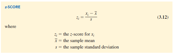
The z-score is often called the standardized value. The z-score, z_t, can be interpreted as the number of standard deviations x_i is from the mean X. For example, z₁ = 1.2 would indicate that x₁ is 1.2 standard deviations greater than the sample mean. Similarly, z₂ = -.5 would indicate that x₂ is .5, or 1/2, standard deviation less than the sample mean. A z-score greater than zero occurs for observations with a value greater than the mean, and a z-score less than zero occurs for observations with a value less than the mean. A z-score of zero indicates that the value of the observation is equal to the mean.

The z-score for any observation can be interpreted as a measure of the relative location of the observation in a data set. Thus, observations in two different data sets with the same z-score can be said to have the same relative location in terms of being the same number of standard deviations from the mean.

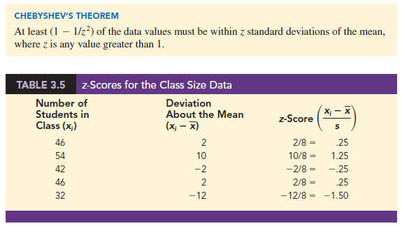
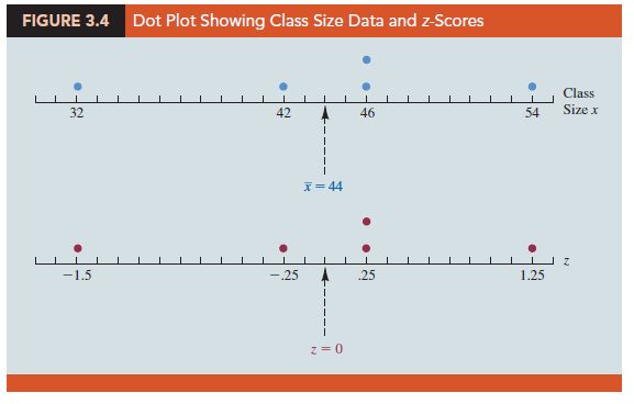
The z-scores for the class size data from Section 3.1 are computed in Table 3.5. Recall the previously computed sample mean, x = 44, and sample standard deviation, s = 8. The z-score of -1.50 for the fifth observation shows it is farthest from the mean; it is 1.50 stan­dard deviations below the mean. Figure 3.4 provides a dot plot of the class size data with a graphical representation of the associated z-scores on the axis below.

3. Chebyshev’s Theorem

Chebyshev’s theorem enables us to make statements about the proportion of data values that must be within a specified number of standard deviations of the mean.

Some of the implications of this theorem, with z = 2, 3, and 4 standard deviations, follow.

• At least .75, or 75%, of the data values must be within z = 2 standard deviations of the mean.
• At least .89, or 89%, of the data values must be within z = 3 standard deviations of the mean.
• At least .94, or 94%, of the data values must be within z = 4 standard deviations of the mean.

For an example using Chebyshev’s theorem, suppose that the midterm test scores for 100 students in a college business statistics course had a mean of 70 and a standard devia­tion of 5. How many students had test scores between 60 and 80? How many students had test scores between 58 and 82?

For the test scores between 60 and 80, we note that 60 is two standard deviations below the mean and 80 is two standard deviations above the mean. Using Chebyshev’s theorem, we see that at least .75, or at least 75%, of the observations must have values within two standard de­viations of the mean. Thus, at least 75% of the students must have scored between 60 and 80.

For the test scores between 58 and 82, we see that (58 – 70)/5 = -2.4 indicates 58 is 2.4 standard deviations below the mean and that (82 – 70)/5 = +2.4 indicates 82 is 2.4 standard deviations above the mean. Applying Chebyshev’s theorem with z =4, we have

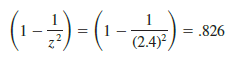
At least 82.6% of the students must have test scores between 58 and 82.

4. Empirical Rule

One of the advantages of Chebyshev’s theorem is that it applies to any data set regardless of the shape of the distribution of the data. Indeed, it could be used with any of the distribu­tions in Figure 3.3. In many practical applications, however, data sets exhibit a symmetric mound-shaped or bell-shaped distribution like the one shown in blue in Figure 3.5. When the data are believed to approximate this distribution, the empirical rule can be used to determine the percentage of data values that must be within a specified number of standard deviations of the mean.

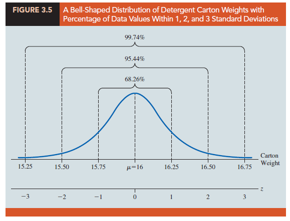
For example, liquid detergent cartons are filled automatically on a production line. Filling weights frequently have a bell-shaped distribution. If the mean filling weight is 16 ounces and the standard deviation is .25 ounces, we can use the empirical rule to draw the following conclusions.

• Approximately 68% of the filled cartons will have weights between 15.75 and 16.25 ounces (within one standard deviation of the mean).
• Approximately 95% of the filled cartons will have weights between 15.50 and
• ounces (within two standard deviations of the mean).
• Almost all filled cartons will have weights between 15.25 and 16.75 ounces (within three standard deviations of the mean).

Can we use this information to say anything about how many filled cartons will:

• weigh between 16 and 16.25 ounces?
• weigh between 15.50 and 16 ounces?
• weigh less than 15.50 ounces?
• weigh between 15.50 and 16.25 ounces?

If we recognize that the normal distribution is symmetric about its mean, we can answer each of the questions in the previous list, and we will be able to determine the following:

• Since the percentage of filled cartons that will weigh between 15.75 and 16.25 is approximately 68% and the mean 16 is at the midpoint between 15.75 and 16.25, the percentage of filled cartons that will weigh between 16 and 16.25 ounces is approxi­mately (68%)/2 or approximately 34%.
• Since the percentage of filled cartons that will weigh between 15.50 and 16.50 is approximately 95% and the mean 16 is at the midpoint between 15.50 and 16.50, the percentage of filled cartons that will weigh between 15.50 and 16 ounces is approxi­mately (95%)/2 or approximately 47.5%.
• We just determined that the percentage of filled cartons that will weigh between
• and 16 ounces is approximately 47.5%. Since the distribution is symmetric about its mean, we also know that 50% of the filled cartons will weigh below 16 ounces. Therefore, the percentage of filled cartons with weights less than
• ounces is approximately 50% – 47.5% or approximately 2.5%.
• We just determined that approximately 47.5% of the filled cartons will weigh be­tween 15.50 and 16 ounces, and we earlier determined that approximately 34% of the filled cartons will weigh between 16 and 16.25 ounces. Therefore, the percentage of filled cartons that will weigh between 15.50 and 16.25 ounces is approximately 47.5% + 34% or approximately 81.5%.

In Chapter 6 we will learn to work with noninteger values of z to answer a much broader range of these types of questions.

5. Detecting Outliers

Sometimes a data set will have one or more observations with unusually large or unusually small values. These extreme values are called outliers. Experienced statisticians take steps to identify outliers and then review each one carefully. An outlier may be a data value that has been incorrectly recorded. If so, it can be corrected before further analysis. An outlier may also be from an observation that was incorrectly included in the data set; if so, it can be removed. Finally, an outlier may be an unusual data value that has been recorded cor­rectly and belongs in the data set. In such cases it should remain.

Standardized values (z-scores) can be used to identify outliers. Recall that the empiri­cal rule allows us to conclude that for data with a bell-shaped distribution, almost all the data values will be within three standard deviations of the mean. Hence, in using z-scores to identify outliers, we recommend treating any data value with a z-score less than -3 or greater than +3 as an outlier. Such data values can then be reviewed for accuracy and to determine whether they belong in the data set.

Refer to the z-scores for the class size data in Table 3.5. The z-score of -1.50 shows the fifth class size is farthest from the mean. However, this standardized value is well within the – 3 to + 3 guideline for outliers. Thus, the z-scores do not indicate that outliers are present in the class size data.

Another approach to identifying outliers is based upon the values of the first and third quartiles (Q₁ and Q₃) and the interquartile range (IQR). Using this method, we first com­pute the following lower and upper limits:

Lower Limit = Q₁ — 1.5(IQR)

Upper Limit = Q₃ + 1.5(IQR)

An observation is classified as an outlier if its value is less than the lower limit or greater than the upper limit. For the monthly starting salary data shown in Table 3.1, Q₁ = 5857.5, Q₃ = 6025, IQR = 167.5, and the lower and upper limits are

Lower Limit = Q₁ — 1.5(IQR) = 5857.5 — 1.5(167.5) = 5606.25

Upper Limit = Q₃ + 1.5(IQR) = 6025 + 1.5(167.5) = 6276.25

Looking at the data in Table 3.1, we see that there are no observations with a starting salary less than the lower limit of 5606.25. But, there is one starting salary, 6325, that is greater than the upper limit of 6276.25. Thus, 6325 is considered to be an outlier using this alter­nate approach to identifying outliers.

Source:  Anderson David R., Sweeney Dennis J., Williams Thomas A. (2019), Statistics for Business & Economics, Cengage Learning; 14th edition.