Moving Averages and Exponential Smoothing in Time Series Analysis

In this section, we discuss three forecasting methods that are appropriate for a time series with a horizontal pattern: moving averages, weighted moving averages, and exponential smoothing. These methods also adapt well to changes in the level of a horizontal pattern such as we saw with the extended gasoline sales time series (Table 17.2 and Figure 17.2). However, without modification they are not appropriate when significant trend, cyclical, or seasonal effects are present. Because the objective of each of these methods is to “smooth out” the random fluctuations in the time series, they are referred to as smoothing methods. These methods are easy to use and generally provide a high level of accuracy for short- range forecasts, such as a forecast for the next time period.

1. Moving Averages

The moving averages method uses the average of the most recent k data values in the time series as the forecast for the next period. Mathematically, a moving average forecast of order k is as follows:

The term moving is used because every time a new observation becomes available for the time series, it replaces the oldest observation in the equation and a new average is computed. As a result, the average will change, or move, as new observations become available.

To illustrate the moving averages method, let us return to the gasoline sales data in Table 17.1 and Figure 17.1. The time series plot in Figure 17.1 indicates that the gasoline sales time series has a horizontal pattern. Thus, the smoothing methods of this section are applicable.

To use moving averages to forecast a time series, we must first select the order, or number of time series values, to be included in the moving average. If only the most recent values of the time series are considered relevant, a small value of k is preferred. If more past values are considered relevant, then a larger value of k is better. As mentioned earlier, a time series with a horizontal pattern can shift to a new level over time. A moving average will adapt to the new level of the series and resume providing good forecasts in k periods.

Thus, a smaller value of k will track shifts in a time series more quickly. But larger values of k will be more effective in smoothing out the random fluctuations over time. So, man­agerial judgment based on an understanding of the behavior of a time series is helpful in choosing a good value for k.

To illustrate how moving averages can be used to forecast gasoline sales, we will use a three-week moving average (k = 3). We begin by computing the forecast of sales in week 4 using the average of the time series values in weeks 1-3.

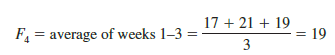
Thus, the moving average forecast of sales in week 4 is 19 or 19,000 gallons of gasoline. Be­cause the actual value observed in week 4 is 23, the forecast error in week 4 is 23 – 19 = 4.

Next, we compute the forecast of sales in week 5 by averaging the time series values in weeks 2-4.

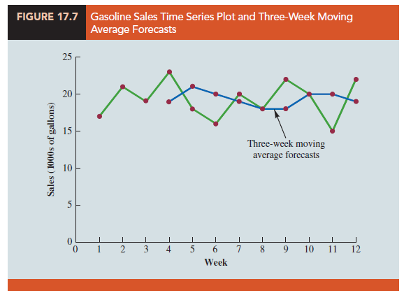
Hence, the forecast of sales in week 5 is 21 and the error associated with this forecast is 18 – 21 = -3. A complete summary of the three-week moving average forecasts for the gasoline sales time series is provided in Table 17.9. Figure 17.7 shows the original time series plot and the three-week moving average forecasts. Note how the graph of the moving average forecasts has tended to smooth out the random fluctuations in the time series.

To forecast sales in week 13, the next time period in the future, we simply compute the average of the time series values in weeks 10, 11, and 12.

Thus, the forecast for week 13 is 19 or 19,000 gallons of gasoline.

Forecast Accuracy In Section 17.2 we discussed three measures of forecast accuracy: MAE, MSE, and MAPE. Using the three-week moving average calculations in Table 17.9, the values for these three measures of forecast accuracy are

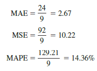
In Section 17.2 we also showed that using the most recent observation as the forecast for the next week (a moving average of order k = 1) resulted in values of MAE = 3.73, MSE = 16.27, and MAPE = 19.24%. Thus, in each case the three-week moving average approach provided more accurate forecasts than simply using the most recent observation as the forecast.

To determine if a moving average with a different order k can provide more accurate forecasts, we recommend using trial and error to determine the value of k that minimizes MSE. For the gasoline sales time series, it can be shown that the minimum value of MSE corresponds to a moving average of order k = 6 with MSE = 6.79. If we are willing to assume that the order of the moving average that is best for the historical data will also be best for future values of the time series, the most accurate moving average forecasts of gasoline sales can be obtained using a moving average of order k = 6.

2. Weighted Moving Averages

In the moving averages method, each observation in the moving average calculation receives the same weight. One variation, known as weighted moving averages, involves selecting a different weight for each data value and then computing a weighted average of the most recent k values as the forecast. In most cases, the most recent observation receives the most weight, and the weight decreases for older data values. Let us use the gasoline sales time series to illustrate the computation of a weighted three-week moving average. We assign a weight of 3/6 to the most recent observation, a weight of 2/6 to the second most recent observation, and a weight of 1/6 to the third most recent observation. Using this weighted average, our forecast for week 4 is computed as follows:

Forecast for week 4 = ¹/₆ (17) + ²/₆ (21) + ³/₆ (19) = 19.33

Note that for the weighted moving average method the sum of the weights is equal to 1.

Forecast Accuracy To use the weighted moving averages method, we must first select the number of data values to be included in the weighted moving average and then choose weights for each of the data values. In general, if we believe that the recent past is a better predictor of the future than the distant past, larger weights should be given to the more recent observations. However, when the time series is highly variable, selecting approxi­mately equal weights for the data values may be best. The only requirement in selecting the weights is that their sum must equal 1. To determine whether one particular combina­tion of number of data values and weights provides a more accurate forecast than another combination, we recommend using MSE as the measure of forecast accuracy. That is, if we assume that the combination that is best for the past will also be best for the future, we would use the combination of number of data values and weights that minimizes MSE for the historical time series to forecast the next value in the time series.

3. Exponential Smoothing

Exponential smoothing also uses a weighted average of past time series values as a fore­cast; it is a special case of the weighted moving averages method in which we select only one weight—the weight for the most recent observation. The weights for the other data values are computed automatically and become smaller as the observations move farther into the past. The exponential smoothing equation follows.

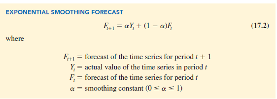
Equation (17.2) shows that the forecast for period t + 1 is a weighted average of the actual value in period t and the forecast for period t. The weight given to the actual value in period t is the smoothing constant a and the weight given to the forecast in period t is 1 – a. It turns out that the exponential smoothing forecast for any period is actually a weighted average of all the previous actual values of the time series. Let us illustrate by working with a time series involving only three periods of data: Y₁, Y₂, and Y₃.

To initiate the calculations, we let F₁ equal the actual value of the time series in period 1; that is, F₁ = Y₁. Hence, the forecast for period 2 is

We see that the exponential smoothing forecast for period 2 is equal to the actual value of the time series in period 1.

The forecast for period 3 is

Finally, substituting this expression for F3 in the expression for F4, we obtain

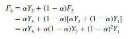
We now see that F₄ is a weighted average of the first three time series values. The sum of the coefficients, or weights, for Y₁, Y₂, and Y₃ equals 1. A similar argument can be made to show that, in general, any forecast F_t+1 is a weighted average of all the previous time series values.

Despite the fact that exponential smoothing provides a forecast that is a weighted aver­age of all past observations, all past data do not need to be saved to compute the forecast for the next period. In fact, equation (17.2) shows that once the value for the smoothing constant a is selected, only two pieces of information are needed to compute the forecast: Y_t, the actual value of the time series in period t, and F_t, the forecast for period t.

To illustrate the exponential smoothing approach, let us again consider the gasoline sales time series in Table 17.1 and Figure 17.1. As indicated previously, to start the calcu­lations we set the exponential smoothing forecast for period 2 equal to the actual value of the time series in period 1. Thus, with Y₁ = 17, we set F₂ = 17 to initiate the computations. Referring to the time series data in Table 17.1, we find an actual time series value in period 2 of Y₂ = 21. Thus, period 2 has a forecast error of 21 – 17 = 4.

Continuing with the exponential smoothing computations using a smoothing constant of a = .2, we obtain the following forecast for period 3:

Once the actual time series value in period 3, Y₃ = 19, is known, we can generate a forecast for period 4 as follows:

Continuing the exponential smoothing calculations, we obtain the weekly forecast values shown in Table 17.10. Note that we have not shown an exponential smoothing forecast or a forecast error for week 1 because no forecast was made. For week 12, we have Y₁₂ = 22 and F₁₂ = 18.48. We can we use this information to generate a forecast for week 13.

Thus, the exponential smoothing forecast of the amount sold in week 13 is 19.18, or 19,180 gallons of gasoline. With this forecast, the firm can make plans and decisions accordingly.

Figure 17.8 shows the time series plot of the actual and forecast time series values. Note in particular how the forecasts “smooth out” the irregular or random fluctuations in the time series.

Forecast Accuracy In the preceding exponential smoothing calculations, we used a smoothing constant of a = .2. Although any value of a between 0 and 1 is acceptable, some values will yield better forecasts than others. Insight into choosing a good value for a can be obtained by rewriting the basic exponential smoothing model as follows:

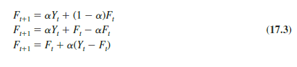
Thus, the new forecast F_t+1 is equal to the previous forecast F_t plus an adjustment, which is the smoothing constant a times the most recent forecast error, Y_t – F_t. That is, the forecast in period t + 1 is obtained by adjusting the forecast in period t by a fraction of the fore­cast error. If the time series contains substantial random variability, a small value of the smoothing constant is preferred. The reason for this choice is that if much of the forecast error is due to random variability, we do not want to overreact and adjust the forecasts too quickly. For a time series with relatively little random variability, forecast errors are more likely to represent a change in the level of the series. Thus, larger values of the smoothing constant provide the advantage of quickly adjusting the forecasts; this allows the forecasts to react more quickly to changing conditions.

The criterion we will use to determine a desirable value for the smoothing constant a is the same as the criterion we proposed for determining the order or number of periods of data to include in the moving averages calculation. That is, we choose the value of a that minimizes the MSE. A summary of the MSE calculations for the exponential smoothing forecast of gasoline sales with a = .2 is shown in Table 17.10. Note that there is one less squared error term than the number of time periods because we had no past values with which to make a forecast for period 1. The value of the sum of squared forecast errors is 98.80; hence MSE = 98.80/11 = 8.98. Would a different value of a provide better results in terms of a lower MSE value? Perhaps the most straightforward way to answer this ques­tion is simply to try another value for a. We will then compare its mean squared error with the MSE value of 8.98 obtained by using a smoothing constant of a = .2.

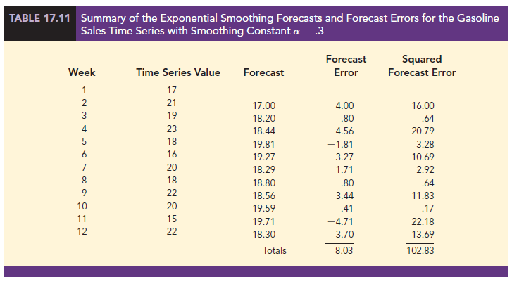
The exponential smoothing results with a = .3 are shown in Table 17.11. The value of the sum of squared forecast errors is 102.83; hence MSE = 102.83/11 = 9.35. With MSE = 9.35, we see that, for the current data set, a smoothing constant of a = .3 results in less forecast accuracy than a smoothing constant of a = .2. Thus, we would be inclined to prefer the original smoothing constant of a = .2. Using a trial-and-error calculation with other values of a, we can find a “good” value for the smoothing constant. This value can be used in the exponential smoothing model to provide forecasts for the future. At a later date, after new time series observations are obtained, we analyze the newly collected time series data to determine whether the smoothing constant should be revised to provide better forecasting results.

Source:  Anderson David R., Sweeney Dennis J., Williams Thomas A. (2019), Statistics for Business & Economics, Cengage Learning; 14th edition.