Multiple Regression with SPSS – Problem 6.1: Using the Simultaneous Method to Compute Multiple Regression

To reiterate, the purpose of multiple regression is to predict an interval (or scale) dependent variable from a combination of several interval/scale and/or dichotomous independent/predictor variables. In the following assignment, we will see if math achievement can be predicted better from a combination of several of our other variables, such as the motivation scale, grades in high school, and mother’s and father’s education. In Problems 6.1 and 6.5, we will run the multiple regression using alternate methods provided by SPSS. In Problem 6.1, we will assume that all seven of the predictor variables are important and that we want to see what is the highest possible multiple correlation of these variables with the dependent variable. For this purpose, we will use the method that SPSS calls Enter (often called simultaneous regression), which tells the computer to consider all the variables at the same time. In Problem 6.3, we will use the hierarchical method.

• How well does the combination of motivation, competence, pleasure, grades in high school, father’s education, mother’s education, and gender predict math achievement?

In this problem, the computer will enter/consider all the variables into the model at the same time. Also, we will ask which of these seven predictors contribute significantly to the multiple correlation/regression.

It is a good idea to check the correlations among the predictor variables prior to running the multiple regression to determine if the predictors are correlated such that multicollinearity is highly likely to be a problem. This is especially important to do when one is using a relatively large set of predictors and/or if, for empirical or conceptual reasons, one believes that some or all of the predictors might be highly correlated. If variables are highly correlated (e.g., correlated at .50 or .60 and above), then one might decide to combine (aggregate) them into a composite variable or eliminate one or more of the highly correlated variables if the variables do not make a meaningful composite variable. For this example, we will check correlations between the variables to see if there might be multicollinearity problems. We typically also would create a scatterplot matrix to check the assumption of linear relationships of each predictor with the dependent variable and a scatterplot between the predictive equation and the residual to check for the assumption that these are uncorrelated. In this problem, we will not do so because we will show you how to do these assumption checks in Problem 6.2.

• Click on Analyze →Correlate → Bivariate… The Bivariate Correlations window will appear.
• Select the variables motivation scale, competence scale, pleasure scale, grades in h.s., father’s education, mother’s education, and gender and click them over to the Variables
• Click on Options. Under Missing Values click on Exclude cases listwise.
• Click on Continue and then on OK. A correlation matrix like the one in Output 6.1a will appear.

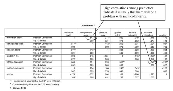
Output 6.1a: Correlation Matrix

CORRELATIONS /VARIABLES=motivation competence pleasure grades faed maed gender /PRINT=TWOTAIL NOSIG /MISSING=LISTWISE.

Correlations

High correlations among predictors indicate it is likely that there will be a problem with multicollinearity.

Interpretation of Output 6.1a

The correlation matrix indicates large correlations between motivation and competence and between mother’s education and father’s education. If predictor variables are highly correlated and conceptually related to one another, we would usually aggregate them, not only to reduce the likelihood of multicollinearity but also to reduce the number of predictors, which typically increases power. If predictor variables are highly correlated but conceptually are distinctly different (so aggregation does not seem appropriate), we might decide to eliminate the less important predictor before running the regression. However, if we have reasons for wanting to include both variables as separate predictors, we should run collinearity diagnostics to see if collinearity actually is a problem.

For this problem, we also want to show how the collinearity problems created by these highly correlated predictors affect the Tolerance values and the significance of the beta coefficients, so we will run the regression without altering the variables. To run the regression, follow the steps below:

• Click on the following: Analyze → Regression → Linear… The Linear Regression window ( 6.1) should appear.
• Select math achievement and click it over to the Dependent box (dependent variable).
• Next select the variables motivation scale, competence scale, pleasure scale, grades in h.s., father’s education, mother’s education, and gender and click them over to the Independent(s) box (independent variables).
• Under Method, be sure that Enter is selected.

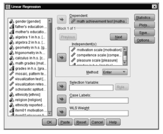
Fig.6.1.Linear regression.

• Click on Statistics, click on Estimates (under Regression Coefficients), and click on Model fit, Descriptives, Part and partial correlations, and Collinearity diagnostics (see Fig. 6.2).

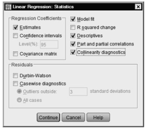
Fig.6.2.Linear regression: Statistics.

• Click on Continue.
• Click on OK.

Compare your output and syntax to Output 6.1b.

Output 6.1b: Multiple Linear Regression, Method = Enter

REGRESSION

/DESCRIPTIVES MEAN STDDEV CORR SIG N

/MISSING LISTWISE

/STATISTICS COEFF OUTS R ANOVA COLLIN TOL ZPP

/CRITERIA=PIN(.05) POUT(.10)

/NOORIGIN

/DEPENDENT mathach

/METHOD=ENTER motivatn competnc pleasure grades faed maed gend.

Regression

Interpretation of Output 6.1b

First, the output provides the usual Descriptive Statistics for all eight variables. Note that N is 69 because six participants are missing a score on one or more variables. Multiple regression uses only the participants who have complete data for all the variables. The next table is a correlation matrix similar to the one in Output 6.1a. Note that the first column shows the correlations of the other variables with math achievement and that motivation, competence, grades in high school, father’s education, mother’s education, and gender are all significantly correlated with math achievement. As we observed before, several of the predictor/independent variables are highly correlated with each other, that is, competence and motivation (.517) and mother’s education and father’s education (.649).

The Model Summary table shows that the multiple correlation coefficient (R), using all the predictors simultaneously, is .65 (R² = .43), and the adjusted R² is .36, meaning that 36% of the variance in math achievement can be predicted from gender, competence, etc. combined. Note that the adjusted R² is lower than the unadjusted R². This is, in part, related to the number of variables in the equation. The adjustment is also affected by the magnitude of the effect and the sample size. Because so many independent variables were used, especially given difficulties with collinearity, a reduction in the number of variables might help us find an equation that explains more of the variance in the dependent variable. It is helpful to use the concept of parsimony with multiple regression and use the smallest number of predictors needed.

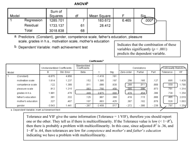
Tolerance and V1F give the same information (Tolerance = 1/VIF), therefore you should report one or the other. They tell us if there is multicollinearity. If the Tolerance value is low (< 1-R~), then there is probably a problem with multicollinearity, In this case, since adjusted R’ is .36, and I R^: is .64. then tolerances are low for competence and mother’s and father’s education indicating we have a problem with multicollinearity.

Interpretation of Output 6.1b continued The ANOVA table shows that F = 6.47 and is significant. This indicates that the combination of the predictors significantly predict math achievement.

One of the most important tables is the Coefficients table. It provides the standardized beta coefficients, which are interpreted similarly to correlation coefficients or factor weights (see Chapter 4). The t value and the Sig opposite each independent variable indicates whether that variable is significantly contributing to the equation for predicting math achievement from the whole set of predictors. Thus, h.s. grades and gender, in this example, are the only variables that are significantly adding anything to the prediction when the other five variables are also entered. It is important to note that all the variables are being considered together when these values are computed. Therefore, if you delete one of the predictors that is not significant, it can affect the size of the betas and levels of significance for other predictors. This is particularly true if high collinearity exists.

Another important aspect of the Coefficients table are the Correlations: zero order (bivariate), partial and part. The Partial correlation values, when they are squared, give us an indication of the amount of unique variance (variance that is not explained by any of the other variables) in the outcome variable (math achievement) predicted by each independent variable. In the output, we can see that competence explains the least amount of unique variance (.011² < 1%) and grades in high school explains the most (.454² = 21%).

Moreover, as the Tolerances in the Coefficients table suggest, and as we will see in Problem 6.2, the standardized beta results are somewhat misleading. Although the two parent education measures were significantly correlated with math achievement, they did not contribute to the multiple regression predicting math achievement. What has happened here is that these two measures were also highly correlated with each other, and multiple regression eliminates all overlap between predictors. Thus, neither father’s education nor mother’s education had much to contribute when the other was also used as a predictor. Note that tolerance for each of these variables is < .64 (1-.36), indicating that too much multicollinearity (overlap between predictors) exists. One way to handle multicollinearity is to combine variables that are highly related if that makes conceptual sense. For example, you could make a new variable called parents’ education, as we will for Problem 6.2. Tolerance is also low for competence, if motivation and pleasure also are entered. We will discuss what to do in this case in Problem 6.2.

Interpretation of Output 6.1b continued This table gives you more information about collinearity in the model. Eigenvalues should be close to 1, Variance Proportions should be high for just one variable on each dimension, and Condition Indexes should be under 15. (Usually, 15-30 is usually considered to indicate possible collinearity; over 30 to indicates problematic collinearity). Low eigenvalues and high condition indexes can indicate collinearity difficulties, particularly when more than one variable has a large variance proportion for that dimension. In this example, none of the condition indexes is extremely high, but dimensions 4-8 have low eigenvalues, dimensions 6-8 have somewhat high condition indexes, and both father’s education and mother’s education primarily are explained by the sam e dimension. All of these suggest possible collinearity issues.

Source: Leech Nancy L. (2014), IBM SPSS for Intermediate Statistics, Routledge; 5th edition;

download Datasets and Materials.