The General Structural Equation Model

1. Symbol Notation

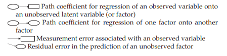
Structural equation models are schematically portrayed using particular configurations of four geometric symbols—a circle (or ellipse), a square (or rectangle), a single-headed arrow, and a double-headed arrow. By conven­tion, circles (or ellipses; CD) represent unobserved latent factors, squares (or rectangles; ) represent observed variables, single-headed arrows (→) represent the impact of one variable on another, and double-headed arrows (^) represent covariances or correlations between pairs of varia­bles. In building a model of a particular structure under study, researchers use these symbols within the framework of four basic configurations, each of which represents an important component in the analytic process. These configurations, each accompanied by a brief description, are as follows:

2. The Path Diagram

Schematic representations of models are termed path diagrams because they provide a visual portrayal of relations that are assumed to hold among the variables under study. Essentially, as you will see later, a path diagram depicting a particular SEM model is actually the graphical equivalent of its mathematical representation whereby a set of equations relates dependent variables to their explanatory variables. As a means of illustrating how the above four symbol configurations may represent a particular causal pro­cess, let me now walk you through the simple model shown in Figure 1.1, which was formulated using Amos Graphics (Arbuckle, 2015).

In reviewing the model shown in Figure 1.1, we see that there are two unobserved latent factors—math self-concept (MSC) and math achieve­ment (MATH)—and five observed variables—three of which are con­sidered to measure MSC (SDQMSC; APIMSC; SPPCMSC), and two to measure MATH (MATHGR; MATHACH). These five observed variables function as indicators of their respective underlying latent factors.

Associated with each observed variable is an error term (err1-err5), and with the factor being predicted (MATH), a residual term (resid1)²; there is an important distinction between the two. Error associated with observed variables represents measurement error, which reflects on their adequacy in measuring the related underlying factors (MSC; MATH). Measurement error derives from two sources: random measurement error (in the psychometric sense) and error uniqueness, a term used to describe error variance arising from some characteristic that is considered to be specific (or unique) to a particular indicator variable. Such error often represents nonrandom (or systematic) measurement error. Residual terms represent error in the prediction of endogenous factors from exogenous factors. For example, the residual term shown in Figure 1.1 represents error in the prediction of MATH (the endogenous factor) from MSC (the exogenous factor).

It is worth noting that both measurement and residual error terms, in essence, represent unobserved variables. Thus, it seems perfectly reasonable that, consistent with the representation of factors, they too should be enclosed in circles. For this reason, then, Amos path diagrams, unlike those associated with most other SEM programs, model these error variables as circled enclo­sures by default.

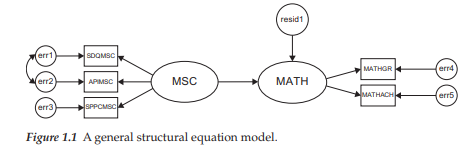
In addition to symbols that represent variables, certain others are used in path diagrams to denote hypothesized processes involving the entire system of variables. In particular, one-way arrows represent struc­tural regression coefficients and thus indicate the impact of one variable on another. In Figure 1.1, for example, the unidirectional arrow pointing toward the endogenous factor, MATH, implies that the exogenous factor MSC (math self-concept) “causes” math achievement (MATH).⁴ Likewise, the three unidirectional arrows leading from MSC to each of the three observed variables (SDQMSC, APIMSC, SPPCMSC), and those leading from MATH to each of its indicators, MATHGR and MATHACH, sug­gest that these score values are each influenced by their respective under­lying factors. As such, these path coefficients represent the magnitude of expected change in the observed variables for every change in the related latent variable (or factor). It is important to note that these observed vari­ables typically represent subscale scores (see, e.g., Chapter 8), item scores (see, e.g., Chapter 4), item pairs (see, e.g., Chapter 3), and/or carefully formulated item parcels (see, e.g., Chapter 6).

The one-way arrows pointing from the enclosed error terms (err1-err5) indicate the impact of measurement error (random and unique) on the observed variables, and that from the residual (residl) indicates the impact of error in the prediction of MATH. Finally, as noted earlier, curved two-way arrows represent covariances or correlations between pairs of variables. Thus, the bidirectional arrow linking errl and err2, as shown in Figure 1.1, implies that measurement error associated with SDQMSC is correlated with that associated with APIMSC.

3. Structural Equations

As noted in the initial paragraph of this chapter, in addition to lending themselves to pictorial description via a schematic presentation of the causal processes under study, structural equation models can also be represented by a series of regression (i.e., structural) equations. Because (a) regression equations represent the influence of one or more variables on another, and (b) this influence, conventionally in SEM, is symbolized by a single-headed arrow pointing from the variable of influence to the variable of interest, we can think of each equation as summarizing the impact of all relevant variables in the model (observed and unobserved) on one specific variable (observed or unobserved). Thus, one relatively simple approach to formulating these equations is to note each variable that has one or more arrows pointing toward it, and then record the sum­mation of all such influences for each of these dependent variables.

To illustrate this translation of regression processes into structural equations, let’s turn again to Figure 1.1. We can see that there are six varia­bles with arrows pointing toward them; five represent observed variables (SDQMSC-SPPCMSC; MATHGR, MATHACH), and one represents an unobserved variable (or factor; MATH). Thus, we know that the regres­sion functions symbolized in the model shown in Figure 1.1 can be sum­marized in terms of six separate equation-like representations of linear dependencies as follows:

MATH = MSC + resid1

SDQMSC = MSC + err1

APIMSC = MSC + err2

SPPCMSC = MSC + err3

MATHGR = MATH + err4

MATHACH = MATH + err5

4. Nonvisible Components of a Model

Although, in principle, there is a one-to-one correspondence between the schematic presentation of a model and its translation into a set of struc­tural equations, it is important to note that neither of these model repre­sentations tells the whole story; some parameters critical to the estimation of the model are not explicitly shown and thus may not be obvious to the novice structural equation modeler. For example, in both the path diagram and the equations just shown, there is no indication that the variances of the exogenous variables are parameters in the model; indeed, such param­eters are essential to all structural equation models. Although researchers must be mindful of this inadequacy of path diagrams in building model input files related to other SEM programs, Amos facilitates the specifica­tion process by automatically incorporating the estimation of variances by default for all independent factors.

Likewise, it is equally important to draw your attention to the specified nonexistence of certain parameters in a model. For example, in Figure 1.1, we detect no curved arrow between err4 and err5, which suggests the lack of covariance between the error terms associated with the observed variables MATHGR and MATHACH. Similarly, there is no hypothesized covariance between MSC and residl; absence of this path addresses the common, and most often necessary, assumption that the predictor (or exogenous) variable is in no way associated with any error arising from the prediction of the criterion (or endogenous) variable. In the case of both examples cited here, Amos, once again, makes it easy for the novice struc­tural equation modeler by automatically assuming these specifications to be nonexistent. (These important default assumptions will be addressed in Chapter 2, where I review the specification of Amos models and input files in detail.)

5. Basic Composition

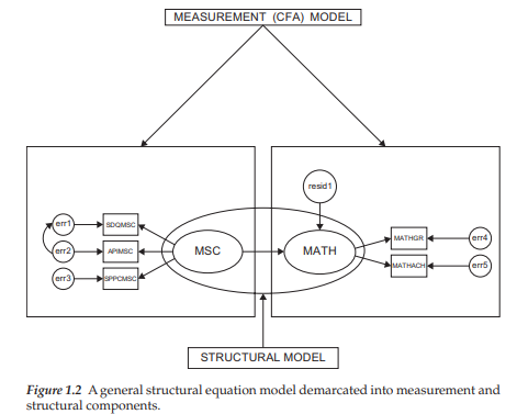
The general SEM model can be decomposed into two submodels: a meas­urement model and a structural model. The measurement model defines relations between the observed and unobserved variables. In other words, it provides the link between scores on a measuring instrument (i.e., the observed indicator variables) and the underlying constructs they are designed to measure (i.e., the unobserved latent variables). The measure­ment model, then, represents the CFA model described earlier in that it specifies the pattern by which each measure loads on a particular factor. In contrast, the structural model defines relations among the unobserved variables. Accordingly, it specifies the manner by which particular latent variables directly or indirectly influence (i.e., “cause”) changes in the val­ues of certain other latent variables in the model.

For didactic purposes in clarifying this important aspect of SEM composition, let’s now examine Figure 1.2, in which the same model pre­sented in Figure 1.1 has been demarcated into measurement and struc­tural components.

Considered separately, the elements modeled within each rectangle in Figure 1.2 represent two CFA models. The enclosure of the two factors within the ellipse represents a full latent variable model and thus would not be of interest in CFA research. The CFA model to the left of the dia­gram represents a one-factor model (MSC) measured by three observed variables (SDQMSC-SPPCMSC), whereas the CFA model on the right rep­resents a one-factor model (MATH) measured by two observed variables (MATHGR, MATHACH). In both cases, the regression of the observed variables on each factor and the variances of both the factor and the errors of measurement are of primary interest; the error covariance would be of interest only in analyses related to the CFA model bearing on MSC.

It is perhaps important to note that, although both CFA models described in Figure 1.2 represent first-order factor models, second- and higher-order CFA models can also be analyzed using Amos. Such hier­archical CFA models, however, are less commonly found in the literature (Kerlinger, 1984). Discussion and application of CFA models in the pre­sent book are limited to first- and second-order models only. (For a more comprehensive discussion and explanation of first- and second-order CFA models, see Bollen, 1989a; Brown, 2006; Kerlinger, 1984.)

6. The Formulation of Covariance and Mean Structures

The core parameters in structural equation models that focus on the analysis of covariance structures are the regression coefficients and the variances and covariances of the independent variables; when the focus extends to the analysis of mean structures, the means and intercepts also become central parameters in the model. However, given that sample data comprise observed scores only, there needs to be some internal mechan­ism whereby the data are transposed into parameters of the model. This task is accomplished via a mathematical model representing the entire system of variables. Such representation systems can, and do, vary with each SEM computer program. Because adequate explanation of the way in which the Amos representation system operates demands knowledge of the program’s underlying statistical theory, the topic goes beyond the aims and intent of the present volume. Thus, readers interested in a com­prehensive explanation of this aspect of the analysis of covariance struc­tures are referred to the following texts and monograph: Bollen (1989a), Saris & Stronkhorst (1984), Long (1983b).

In this chapter, I have presented you with a few of the basic concepts associated with SEM. As with any form of communication, one must first understand the language before being able to understand the message conveyed, and so it is in comprehending the specification of SEM mod­els. Now that you are familiar with the basic concepts underlying struc­tural equation modeling, we can turn our attention to the specification and analysis of models within the framework of the Amos program. In the next chapter, then, I provide you with details regarding the specifica­tion of models within the context of the program’s graphical interface as well as a new feature that allows for such specification in table (or spread­sheet) format. Along the way, I show you how to use the Toolbox facil­ity in building models, review many of the drop-down menus, and detail specified and illustrated components of three basic SEM models. As you work your way through the applications included in this book, you will become increasingly more confident in both your understanding of SEM, and in using the Amos program. So, let’s move on to Chapter 2 and a more comprehensive look at SEM modeling with Amos.

Source: Byrne Barbara M. (2016), Structural Equation Modeling with Amos: Basic Concepts, Applications, and Programming, Routledge; 3rd edition.