In Problem 6.2, we will use the combined/average of the two variables, mother’s education and father’s education, and then recompute the multiple regression after omitting competence and pleasure.
We combined father’s education and mother’s education because it makes conceptual sense and because these two variables are quite highly related (r = .65). We know that entering them as two separate variables created problems with multicollinearity because tolerance levels were low for these two variables, and, despite the fact that both variables were significantly and substantially correlated with math achievement, neither contributed significantly to predicting math achievement when taken together.
When it does not make sense to combine the highly correlated variables, one can eliminate one or more of them. Because the conceptual distinction between motivation, competence, and pleasure was important for us and because motivation was more important to us than competence or pleasure, we decided to delete the latter two scales from the analysis. We wanted to see if motivation would contribute to the prediction of math achievement if its contribution was not canceled out by competence and/or pleasure. Motivation and competence are so highly correlated that they create problems with multicollinearity. We eliminate pleasure as well, even though its tolerance is acceptable, because it is virtually uncorrelated with math achievement, the dependent variable, yet it is correlated with motivation and competence and because the Collinearity Diagnostics table indicates that it is contributing to the collinearity difficulties. Given its low correlation with math achievement, it is unlikely to contribute meaningfully to the prediction of math achievement, and its inclusion would serve only to reduce power and potentially reduce the predictive power of motivation. It would be particularly important to eliminate a variable such as pleasure if it were more strongly correlated with another predictor that remains in the equation, as this can lead to particularly misleading results.
- Rerun Problem 6.1 using the parents’ education variable (pareduc) instead of faed and maed and omitting the competence and pleasure scales.
First, we created a matrix scatterplot (as in Chapter 2) to see if the variables are related to each other in a linear fashion. You can use the syntax in Output 6.2 or use the Analyze → Scatter windows as shown below.
- Click on Graphs → Legacy Dialogs → Scatter/Dot…
- Select Matrix Scatter and click on Define.
- Move math achievement, motivation, grades, parents’ education, and gender into the Matrix Variables: box.
- Click on Options. Check to be sure that Exclude cases listwise is selected.
- Click on Continue and then OK.
Then run the regression using the following steps:
- Click on the following: Analyze → Regression → Linear… The Linear Regression window ( 6.1) should appear. This window may still have the variables moved over to the Dependent and Independent(s) boxes. If so, click on Reset.
- Move math achievement into the Dependent
- Next select the variables motivation, grades in h.s., parents’ education, and gender and move them into the Independent(s) box (independent variables).
- Under Method, be sure that Enter is selected.
- Click on Statistics, click on Estimates (under Regression Coefficients), and click on Model fit, Descriptives, and Collinearity diagnostics (see 6.2).
- Click on Continue.
Then, we added a plot to the multiple regression to see the relationship of the predictors and the residual. To make this plot follow these steps:
- Click on .. (in Fig. 6.1 to get Fig. 6.3).
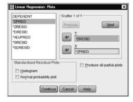
Fig.6.3. Linear regression: Plots.
- Move ZRESID to the Y: box.
- Move ZPRED to the X: box. This enables us to check the assumption that the predictors and residual are uncorrelated.
- Click on Continue.
- Click on OK.
To make the residual plot easier to read, we added a reference line at 0. To do this, follow the steps below:
- Double click on the residual plot. The Chart Editor window will open.
- Click on Options → Y Axis Reference Line. The Properties window will appear.
- Highlight the number in the box next to Position: and type a 0. We are telling SPSS that we want a reference line positioned at 0 on the Y axis.
- Click on Apply and then Close.
- Close the Chart Editor window.
Refer to Output 6.2 for comparison.
Output 6.2: Multiple Linear Regression with Parents’ Education, Method = Enter
GRAPH
/SCATTERPLOT(MATRIX)=mathach motivation grades parEduc gender /MISSING=LISTWISE.
REGRESSION
/DESCRIPTIVES MEAN STDDEV CORR SIG N
/MISSING LISTWISE
/STATISTICS COEFF OUTS R ANOVA COLLIN TOL ZPP
/CRITERIA=PIN(.05) POUT(.10)
/NOORIGIN
/DEPENDENT mathach
/METHOD=ENTER motivation grades parEduc gender
/SCATTERPLOT=(*ZRESID, *ZPRED).
Graph
The top row shows four scatterplots (relationships) of the dependent variables with each of the predictors. To meet the assumption of linearity, a straight line, as opposed to a curved line, should fit the points relatively well.
Source: Leech Nancy L. (2014), IBM SPSS for Intermediate Statistics, Routledge; 5th edition;
download Datasets and Materials.
14 Sep 2022
27 Mar 2023
16 Sep 2022
16 Sep 2022
27 Mar 2023
14 Sep 2022