Problem 4.2: Principal Components Analysis on Achievement Variables with SPSS

Principal components analysis is most useful if one simply wants to reduce a relatively large number of variables to a smaller number of variables that still capture the same information. In this problem we will look at the initial (unrotated) solution as well as the rotated solution because we might want to use the first, unrotated, principal component to summarize all of the variables if it explains most of the variance rather using multiple, rotated components. This would especially be true if the scree plot suggests a large drop-off after the first component in variance explained (eigenvalues), so we will look at the scree plot too.

4.2 Run a principal components analysis to see how the five “achievement” variables cluster. These variables are grades in h.s., math achievement, mosaic pattern test, visualization test, and scholastic aptitude test – math.

• Click on Analyze → Dimension Reduction → Factor…
• First press Reset.
• Next select the variables grades in h.s., math achievement, mosaic pattern test, visualization test, and scholastic aptitude test – math, similar to what we did in 4.1.
• In the Descriptives window ( 4.2), check Univariate descriptives, Initial solution, Coefficients, Determinant, and KMO and Bartlett’s test of sphericity. Click on Continue.
• In the Extraction window ( 4.3), use the default Method of Principal components. Be sure that unrotated factor solution and Eigenvalues over 1 checked. Also, request a Scree plot (to see if one component would do a good job in summarizing the data or if a different number of components would be preferable to the default based on the criterion of components with eigenvalues over 1).
• Click on Continue.
• In the Rotation window ( 4.4), check Varimax. Under Display, check Rotated solution and Loading plot(s).
• Click on Continue and then OK.

We have requested a principal components analysis for the extraction and some different options for the output to contrast with the earlier one. Compare Output 4.2 with your syntax and output.

Output 4.2: Principal Components Analysis for Achievement Scores

FACTOR

/VARIABLES grades mathach mosaic visual satm

/MISSING LISTWISE

/ANALYSIS grades mathach mosaic visual satm

/PRINT UNIVARIATE INITIAL CORRELATION DET KMO EXTRACTION ROTATION

/PLOT EIGEN ROTATION

/CRITERIA MINEIGEN(1) ITERATE(25)

/EXTRACTION PC

/CRITERIA ITERATE(25)

/ROTATION VARIMAX

/METHOD=CORRELATION.

Factor Analysis

Interpretation of 4.2

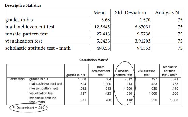
As in 41, the Descriptive Statistics table provides the mean and SD for each item. The Analysis N is important because it tells you how many students have scores on all five of these variables; in this case there is no missing data so the N is 75. The Correlation Matrix shows how each of the five items is related to the other four; note that the mosaic scores are very weakly correlated with the other four variables (-.012 to .213).

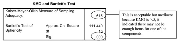
In terms of assumptions, the Determinant is much larger than zero so that is good. The KMO is .615 so mediocre and may be a problem. The Bartlett test is significant (p < .001), which is good and indicates that the correlations are not near zero.

Extraction Method: Principal Component Analysis

Interpretation of 4.2 continued The Total Variance

Explained table shows that there are two components with initial Eigenvalues more than 1.0, although the Eigenvalue for the second component is barely over 1 at 1.01. The first component explains 47.58% of the total variance, but because this is less than 50%, we probably want to rotate more than one component, as shown on the right hand side of this Total Variance Explained table.

The Scree Plot shows the initial Eigenvalues. Note that both the scree plot and the eigenvalues support the conclusion that these five variables can be reduced to two components. Note that the scree plot flattens out after the second component. However, the second component is very poorly defined, relating only to one variable. Thus, one may decide to use only one summary variable, based on all variables except mosaic, or to redo the PCA after omitting mosaic. It usually is best for components to be defined by at least four variables.

The unrotated Component Matrix should not be interpreted. However, if you want to compute only one variable that provides the most information about this set of variables, a linear combination of the variables with high loadings from the first component of the unrotated matrix would be used.

Extraction Method: Principal Component Analysis.

Rotation Method: Varimax with Kaiser Normalization.

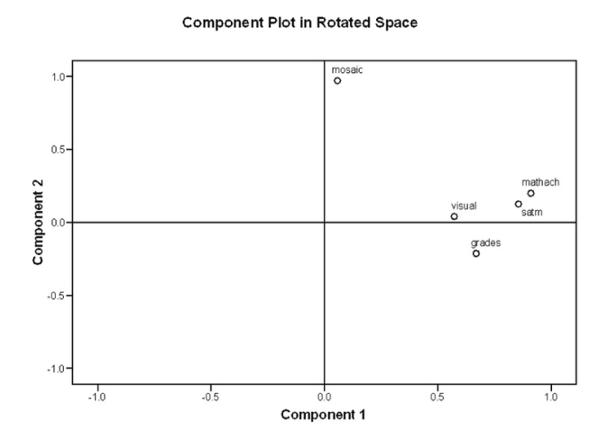
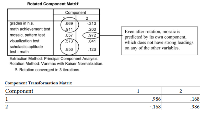
Interpretation of Output 4.2 continued The Rotated Component Matrix, which contains all the loadings (even those < .3) for each component, is similar to the rotated factor matrix in Output 4.1. The Component Plot in Rotated Space gives one a visual representation of the loadings plotted in a 2-dimensional space. The plot shows how closely related the items are to each other and to the two components. This plot of the component loadings shows that math achievement, SATmath, grades in h.s., and visualization test all load highly and positively on the first component. Mosaic has a loading near zero on the first component, but
loads highly on the second.

Also, note that the default setting we used does not sort the variables in the Rotated Component Matrix by magnitude of loadings and does not suppress low loadings. Thus, you have to organize the table yourself; that is, math achievement, scholastic aptitude test, grades in h.s., and visualization, in that order, have high Component 1 loadings, and mosaic is the only variable with a high loading for Component 2.

Researchers usually give names to rotated components in a fashion similar to that used in EFA; however, there is no assumption that this indicates a variable that underlies the measured items. Often, a researcher will aggregate (add or average) the items that define (have high loadings for) each component and use this composite variable in further research. Actually, the same thing is often done with EFA factor loadings; however, the implication of the latter is that this composite variable is an index of the underlying construct.

Example of How to Write About Problem 4.2

Results

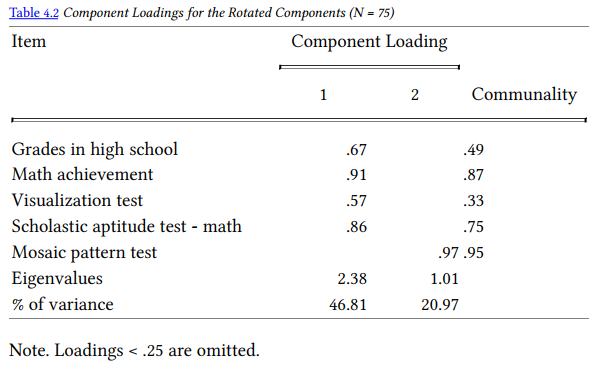
Principal components analysis with varimax rotation was conducted to assess how five “achievement” variables clustered. These variables were grades in h.s., math achievement, mosaic pattern test, visualization test, and scholastic aptitude test – math. (The assumption of independent sampling was met. The assumptions of normality, linear relationships between pairs of variables, and the variables being correlated at a moderate level were checked and mosaic pattern test did not meet the assumptions, in that it was correlated at a low level with each of the other variables.) Two components were rotated, based on the eigenvalues over 1 criterion and the scree plot. After rotation, the first component accounted for 47% of the variance, and the second component accounted for 21% of the variance. Table 4.2 displays the items and component loadings for the rotated components, with loadings less than .30 omitted to improve clarity. Results suggest, in keeping with zero-order correlations, that mosaic pattern test scores are not substantially related to the other measures and should not be aggregated with them but that the other measures form a coherent component.

Source: Leech Nancy L. (2014), IBM SPSS for Intermediate Statistics, Routledge; 5th edition;

download Datasets and Materials.