Multiple Regression with SPSS – Problem 6.3: Hierarchical Multiple Linear Regression

In Problem 6.3, we will use the hierarchical approach, which is used when you want to enter the variables in a series of blocks or groups. This enables the researcher to see if each new group of variables adds anything to the prediction produced by the previous blocks of variables. This approach is an appropriate method to use when the researcher has a priori ideas about how the predictors go together to predict the dependent variable. In our example, we will enter gender first and then see if motivation, grades in h.s., parents’ education, and math courses taken make an additional contribution. This method is intended to control for or eliminate the effects of gender on the prediction.

6.3 If we control for gender differences in math achievement, do any of the other variables significantly add anything to the prediction over and above what gender contributes?

We will include all of the variables from the previous problem; however, this time we include math courses taken, and we will enter the variables in two separate blocks to see how motivation, grades in high school, parents’ education, and math courses taken improve on prediction from gender alone.

• Click on the following: Analyze → Regression → Linear…
• Click on Reset.
• Select math achievement and click it over to the Dependent box (dependent variable).
• Next, select gender and move it over to the Independent(s) box (independent variables).
• Select Enter as your Method (see 6.4).

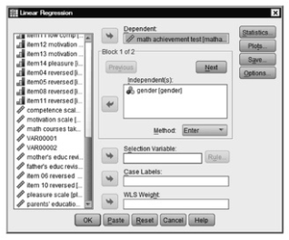
Fig.6.4.Linear regression.

• Click on Next beside Block 1 of 1. You will notice it changes to Block 2 of 2.
• Then move motivation scale, grades in h.s., parents’ education, and math courses taken to the Independent(s) box (independent variables).
• Under Method, select Enter. The window should look like Fig. 6.5.

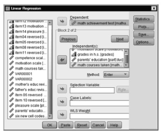
Fig.6.5.Hierarchical regression.

• Click on Statistics, click on Estimates (under Regression Coefficients), and click on Model fit and R squared change (See 6.2.).
• Click on Continue.
• Click on OK.

Compare your output and syntax to Output 6.3.

Output 6.3: Hierarchical Multiple Linear Regression

REGRESSION

/MISSING LISTWISE

/STATISTICS COEFF OUTS R ANOVA CHANGE

/CRITERIA=PIN(.05) POUT(.10)

/NOORIGIN

/DEPENDENT mathach

/METHOD=ENTER gender

/METHOD=ENTER motivation grades parEduc mathcrs.

Regression

Interpretation of Output 6.3

We rechecked the assumptions for this problem, because we added the variable math courses taken. All the assumptions were met. The Descriptives and Correlations tables would have been the same (except for the addition of the variable math courses taken) as those in Problem 6.2 if we had checked the Descriptive box in the Statistics window. The other tables in this output are somewhat different than the previous two outputs. This difference is because we entered the variables in two steps. Therefore, this output has two models listed, Model 1 and Model 2. The information in Model 1 is for gender predicting math achievement. The information in Model 2 is gender plus motivation, grades in h.s., parents’ education, and math courses taken predicting math achievement. In the Model Summary table, we have three new and important pieces of information: R² change, F change, and Sig. F change. The R² change tells you how much the R² increases when you add the new predictors entered in the second step (Model 2). The F change, and Sig. F change for Model 2 tell you whether this change is statistically significant; i.e., whether the additional variables significantly improved on the first model that had only gender as a predictor. In this case, the change improved on the prediction by gender alone, explaining about 56% additional variance. The F change is statistically significant, F(4,67) = 27.23, p < .001. This test is based on the unadjusted R², which does not adjust for the fact that there are more predictors, so it is also useful to compare the adjusted R² for each model, to see if it increases even after the correction for more predictors. The adjusted R² also suggests that Model 2 is better than Model 1 given the large increase in the adjusted R² value from R² = .08 to R² = .63. Furthermore, as we will see in the ANOVA table, Model 2 is highly significant. However, this in itself does not show you that the new model significantly improved on the prior model. It is quite possible for the second model to be significant without its improving to a significant degree on the prior model.

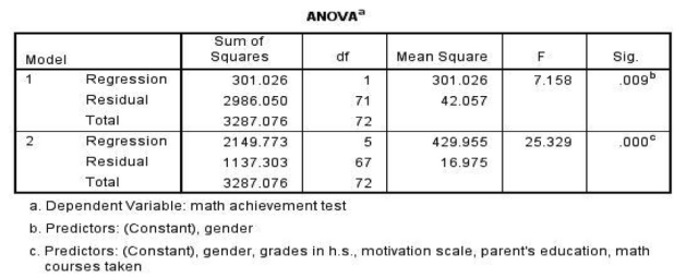
Interpretation of Output 6.3 continued We can see from the ANOVA table that when gender is entered by itself it is a significant predictor of math achievement, F(1,71) = 7.16, p = .009.

However, as you can see from the Coefficients Table below, when the other predictors are entered, gender is no longer a significant predictor of math achievement. This means that boys’ apparent superiority over girls in math achievement could be completely explained by the other predictors. In the final model, only math courses taken significantly predicts math achievement p < .001, and the overall model with the addition of the other predictor variables is significant as well F(5,67) = 25.33, p < .001.

Interpretation of Output 6.3 continued If one wants to make comparisons among predictors to see how much each is contributing to the prediction of the dependent variable, it is best to look at the Standardized Coefficients (Beta weights), especially when variables are on very different scales, as in this example in which gender, a dichotomous variable, is included. On the other hand, the Unstandardized Coefficients give you a better understanding of how the variables, as measured, are weighted to best
predict the outcome, as we will show for Output 6.4 and 6.5.

Included in the Excluded Variables table are the Partial Correlations. As noted in the previous example, these values, when they are squared, give us an indication of the amount of unique variance (variance that is not explained by any of the other variables) each independent variable is explaining in the outcome variable (math achievement). In the output, we can see that motivation explains the least amount of unique variance (.271² = 7%) and math courses taken explains the most (.779² = 61%).

Example of How to Write About Output 6.3

Results

To investigate how well grades in high school, motivation, parents’ education, and math courses taken predict math achievement test scores, after controlling for gender, a hierarchical linear regression was computed. (The assumptions of linearity, normally distributed errors, and uncorrelated errors were checked and met.) Means and standard deviations are presented in Table 6.1. When gender was entered alone, it significantly predicted math achievement, F(1,71) = 7.16, p = .009, adjusted R² = .08. However, as indicated by the R², only 8% of the variance in math achievement could be predicted by knowing the student’s gender. When the other variables were added, they significantly improved the prediction, R² change = .56, F(4,67) = 27.23, p < .001, and gender no longer was a significant predictor. The entire group of variables significantly predicted math achievement, F(5,67) = 25.33, p < .001, adjusted R² = .63. This is a large effect according to Cohen (1988). The beta weights and significance values, presented in Table 6.3, indicates which variable(s) contributes most to predicting math achievement, when gender, motivation, parents’ education, and grades in high school are entered together as predictors. With this combination of predictors, math course taken has the highest beta (.68), and is the only variable that contributes significantly to predicting math achievement.

Source: Leech Nancy L. (2014), IBM SPSS for Intermediate Statistics, Routledge; 5th edition;

download Datasets and Materials.