1. THE INCONSISTENCY OF THE LEAST SQUARES ESTIMATOR
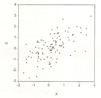
To reproduce Figure 10.2, showing the positive correlation between the x and e generated by the Monte Carlo experiment discussed in the text, first we must “create” the true errors e. In a Monte Carlo world we know the true parameters, and that y is created by
![]()
Therefore we can create the series
![]()
by entering the command
series e = y -1 – x
From the main EViews menu select Quick/Graph. Enter into the Series List dialog box
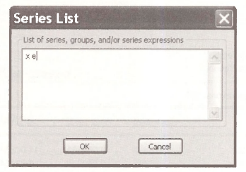
In the Graph Options box choose a basic Scatter diagram. Copying (Ctrl+C) and pasting (Ctrl+V) the figure into our document
To generate Figure 10.3, we must first create
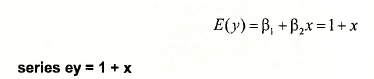
To create
![]()
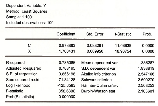
we estimate the simple regression and then obtain the forecasted (predicted) values of y. To estimate the equation enter
Is y c x
The result is
On the regression menu bar select Forecast. In the dialog box enter
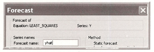
Select X, Y, YHAT, and EY from the workfile, double-click on one of these variables, and select Open Group. After the group is open as a spreadsheet, select View/Graph. In the Graph Options dialog box enter
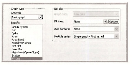
In the Graph Options dialog choose the Line/Symbol tab. Highlight the first series (#1) which is Y. From the Line/Symbol use drop down list choose Symbol only.
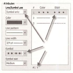
Select series #2, YHAT, and choose Line & Symbol.
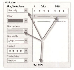
Repeat this for series #3 which is EY.
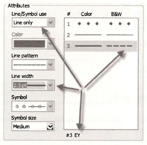
The resulting figure, in black and white, is
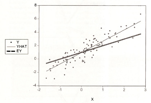
Figure 10.3 shows clearly that the slope of the regression line represented by the fitted dependent variable YHAT overstates the slope of the true population regression function. Hence, ordinary least squares is invalid in cases where x and e are correlated. The variable x is said to be endogenous. The inconsistency of the least squares estimator is due to an endogeneity problem.
2. INSTRUMENTAL VARIABLES/TSLS ESTIMATION
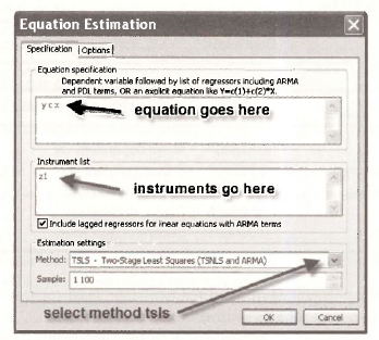
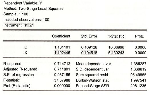
We now turn our attention to the method of instrumental variables estimation, also known as two- stage least squares, described in the text. Instrumental variables estimation produces consistent estimators in the presence of correlation between a random regressor, x, and the error term, e. To obtain the instrumental variables estimates, select Quick/Estimate Equation, and in the Equation Specification dialog box under Estimation Settings, change the Method to: TSLS – Two-Stage Least Squares (TSNLS and ARMA). Next we enter the savings equation in list form Y C X, in the Equation Specification field. Finally, we list the instrument, Zl, in the Instrument List field.
Our results replicate those on page 280 of POE.
Two-stage least squares, using instrumental variables Z1 and Z2, can be carried out by entering on the command line
tsls y c x @ z1 z2
The command is now tsls rather than just Is, and after the equation the instrumental variables are specified after the @-sign. The result is as shown in POE equation (10.27), page 284.
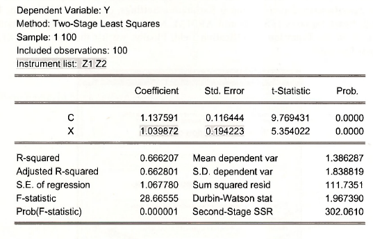
As noted there the estimation procedure is called two-stage least squares because it can actually be implemented using two least squares estimations.
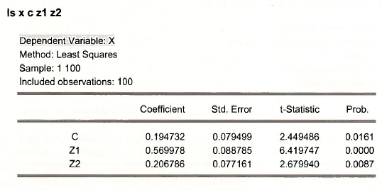
The first stage is a least squares regression of Aon the instruments Z1 and Z2.
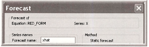
Save this estimated regression with the Name RED_FORM which stands for reduced form.. Select Forecast on the regression menu bar.
Now estimate a least squares regression of Y on XHAT using
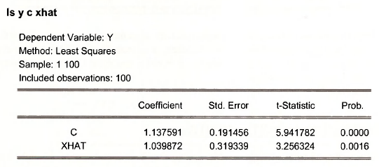
The estimated coefficients using this method are correct (compare them to POE (10.27)) but the standard errors Std. Error are incorrect. Thus two-stage least squares should not actually be implemented this way. Always use the proper tsls procedure.
3. THE HAUSMAN TEST
Here we conduct the Hausman Test for correlation between an explanatory variable, x, and the error term. We continue with the simulated data example. We enter the following commands in the EViews command window:
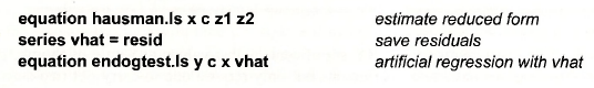
The results are on the next page.
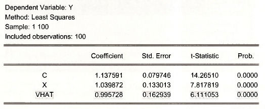
Note that the t-statistic for the coefficient on the residuals from the step one regression is 6.11 and the p-value of this test clearly shows that the /-statistic is statistically significant at the 1% level, so we reject the null hypothesis of no correlation between x and the error term e in favor of the alternative that* and e are correlated.
4. TEST FOR WEAK INSTRUMENTS
A requirement of good instrumental variables is that they be correlated with the right-hand side variable x, which is correlated with the error e. To test this we can examine the reduced form equation. Here consider the reduced form regression of* on the instruments Z1 and Z2.
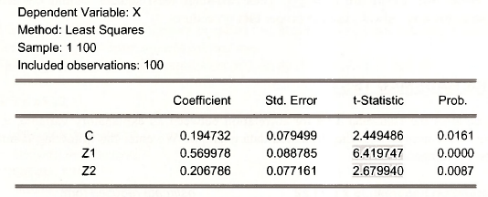
The key is that the instruments are VERY significant, with /-values as a rule of thumb, greater than 3.3. In this case, we have two instruments but only require one to carry out two-stage least squares. Thus we can test the joint null hypothesis that the coefficients of the instruments are zero using an F-test. The alternative hypothesis is that at least one of the two reduced form parameters is not zero, which is exactly what we need.
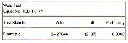
In the regression window of the RED FORM select View/Coefficient Tests/Wald – Coefficient Restrictions. In the dialog box enter
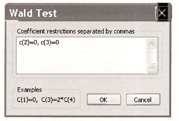
The test result shows that we strongly reject the null hypothesis, and we can conclude that at least one of the reduced form parameters is not zero. Also the F-value is 24.28, which exceeds the rule of thumb guideline of F > 10.
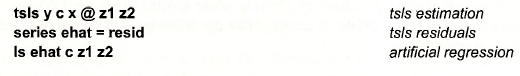
5. TEST INSTRUMENT VALIDITY
In addition to being strongly correlated to the variable x, the instruments must be uncorrelated with the error term e. Because we need one instrument to carry out two-stage least squares estimation, we can only check the validity of this condition for the surplus instruments. In the econometrics literature this is called a test of the over-identifying restrictions, and the test is often called the Sargan test. While there are several variants of this test, we will show a version that is based on the two-stage least squares residuals. We compute the TSLS residuals and regress them on all available instrumental variables. The test statistic is NR2 from this regression, where N is the sample size and R~ is the usual goodness-of-fit measure. If the surplus instruments are valid, the statistic has an asymptotic chi-square distribution with degrees of freedom equal to the number of surplus instruments. The validity of the surplus instruments is rejected if the test statistic value NR2 is greater than the critical value from the chi-square distribution.
The steps are
The results are on the following page.
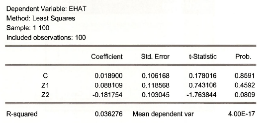
The R2 from this regression is .03628, and NR2 = 3.628. The .05 critical value for the chi-square distribution with one degree of freedom is 3.84, thus we fail to reject the validity of the surplus instrumental variable.
6. A WAGE EQUATION
In Chapter 10.2 we introduced an important example, the estimation of the relationship between wages, specifically \og(WAGE), and years of education (EDUC). We will use the data on married women in the workfile mroz,wfl to examine this relationship. Open this workfile
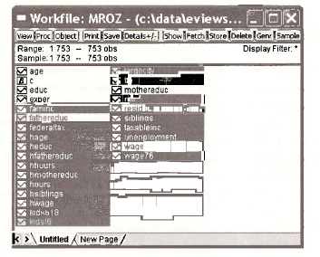
If you are using the EViews 6 Student Version you will get a message saying the workfile is too large. Select all the variable shown above by clicking while holding down the Ctrl-key. Right- click in the blue area, and select Delete. A message like the following will appear, depending on which variable you selected first.

Click Yes to All. You will find the cheerful message

Save the workfile under a new name, such as mroz chaplO.wfl.
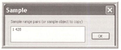
A second problem is that in the data only the first 428 women have wage data. The remainder have WAGE = 0 because they do not participate in the labor market. In the workfile window select the Sample button.
![]()
Fill in the dialog box to include in the estimation sample only the first 428 observations.
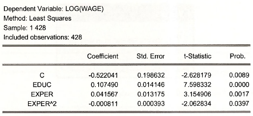
Now we can estimate the equation
![]()
The command is
Is log(wage) c educ exper experˆ2
The result matches those on POE page 281. As noted in POE the concern is that the variable EDUC might be correlated with factors in the error term, such as ability. If that is the case, then the least squares estimator is biased and the bias will not disappear even if the sample size becomes very large.
To implement two-stage least squares we first obtain the reduced form equation, adding mother’s education MOTHEREDUC as an instrumental variable.
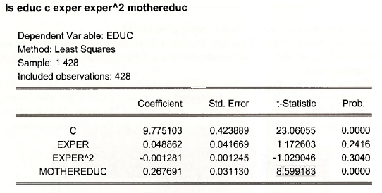
Note that the instrumental variable MOTHEREDUC is very significant, with a /-value of 8.6, indicating that this variable is strongly correlated with EDUC.
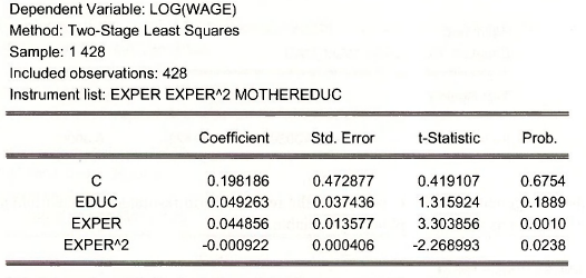
Now implement TSLS. Select Quick/Estimate Equation. The Equation specification is
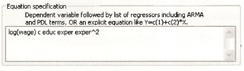
The Instrument list must include all the variables that are NOT correlated with the error term. These variables are said to be exogenous.
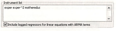
The estimation settings are
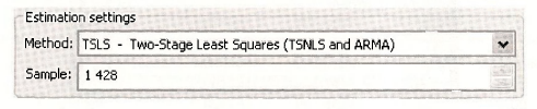
Click OK.
If we use both MOTHEREDUC and FATHEREDUC as instrumental variables the estimated reduced form is obtained using
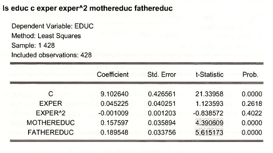
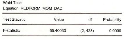
Both instruments are strongly related to the woman’s education EDUC. To test their joint significance select View/Coefficient Tests/Wald – Coefficient Restrictions. In the dialog box enter
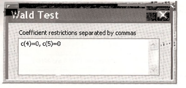
The result shows an F value of 55.4, giving strong evidence that at least one of the instruments has a non-zero coefficient in the reduced form equation.
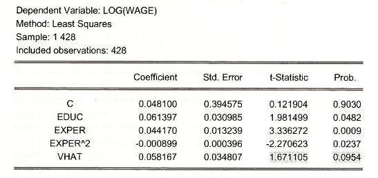
To test the endogeneity of EDUC we obtain the reduced form residuals and then include them in the wage equation as an extra explanatory variable.
series vhat = resid
Is log(wage) c educ exper experˆ2 vhat
The estimation results show that the variable VHAT has a p-value of 0.0954, which is not strong evidence that EDUC is endogenous.
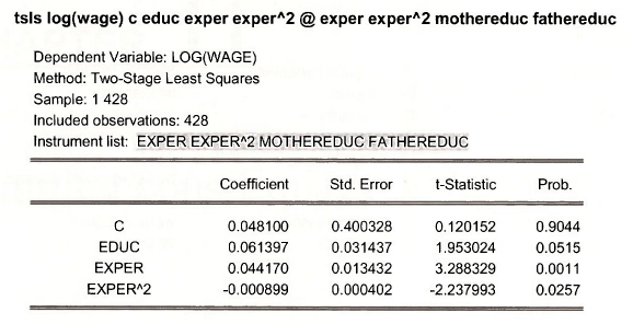
Two-stage least squares estimates can be obtained with the command
To test the validity of the surplus instrumental variable we save the TSLS residuals, and regress them on all the instrumental variables.
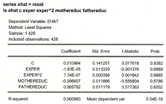
For the artificial regression R2 = .000883, and the test statistic value is
NR2 = 428 x.000883 = .3779
The .05 critical value for the chi-square distribution with one degree of freedom is 3.84, thus we fail to reject the surplus instrument as valid. With this result we are reassured that our instrumental variables estimator for the wage equation is consistent.
Source: Griffiths William E., Hill R. Carter, Lim Mark Andrew (2008), Using EViews for Principles of Econometrics, John Wiley & Sons; 3rd Edition.
20 Sep 2021
20 Sep 2021
20 Sep 2021
20 Sep 2021
20 Sep 2021
20 Sep 2021