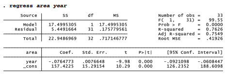
After any regression, the predict command can obtain not only predicted values, but also residuals and other post-estimation case statistics — statistics that have separate values for each observation in the data. Switching to a different example for this section, we will look at the simple regression of September Arctic sea ice area on year (using Arctic9.dta). A downward trend averaging -.076, or roughly 76,000 km2 per year, explains 75% of the variance in area over these years (1979-2011).

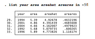
We can create a new variable named areahat, containing predicted values from this regression, and areares, containing residuals, through the post-regression command predict. Predicted values have the same mean as the original y variable. Residuals have a mean of zero (-1.38e-09 = -1.38*10-9 = 0). Note use of a wild-card symbol in the summarize command: area* means all variable names that begin with “area”.

The predicted values and residuals can be analyzed like any other variables. For example, we can test residuals for normality to check on the normal-errors assumption. In this example, a skewness-kurtosis test (sktest) shows that the residuals distribution is not significantly different from normal (p = .45).

Graphing predicted values against year traces the regression line (Figure 7.9).

Residuals contain information about where the model fits poorly, which is helpful for diagnostic or troubleshooting analysis. Such analysis might begin just by sorting and examining the residuals. Negative residuals occur when our model overpredicts the observed values. That is, in certain years the ice area is lower than we might expect based on the overall trend. To list the years with the five lowest residuals, type

Three of the five lowest residuals occurred in the most recent five years, indicating that our trend line overestimates recent ice area.
Positive residuals occur when actual y values are higher than predicted. Because the data already have been sorted by e, to list the five highest residuals we add the qualifier in -5/l. “-5” in this qualifier means the 5th-from-last observation, and the letter “el” (note that this is not the number “1”) stands for the last observations. The qualifiers in -5/-1, in 47/l or in 47/51 each could accomplish the same thing.
Again there is a pattern: the highest positive residuals, or years when a linear model predicts less ice than observed, occur in the 1990s through early 2000s. Before going on to other analysis, we should re-sort the data b typing sort year, so they again form an orderly time series.
Graphs of residuals against predicted values, often called residual-versus-fitted or e-versus-yhat plots, provide a useful diagnostic tool. Figure 7.10 shows a such a graph of areares versus areahat, with a horizontal line drawn at 0, the residual mean. Later in this chapter, Figure 7.17 shows another way to draw such plots.

Ideally, residual versus predicted graphs show no pattern at all, like a swarm of bees that is denser in the middle (see texts such as Hamilton 1992a for good and bad examples). There is a pattern visible in Figure 7.10, however. Predictions are too high in the early years, resulting in mostly negative residuals; too low in the middle, resulting in mostly positive residuals; then too high toward the end, where residuals again turn negative. This is the same pattern noticed earlier when we sorted the residuals by size.
The up and down pattern of residuals becomes obvious in Figure 7.11 in which the residual versus predicted graph is overlaid by a lowess curve. Lowess (locally weighted scatterplot
smoothing) regression provides a broadly useful method for detecting patterns in noisy data. It was briefly introduced in Chapter 3 (Figure 3.26), and will be explained in Chapter 8.

This nonlinear pattern in residuals suggests that our linear model was not appropriate for these data. We return to this point in the next section, and again in Chapter 8.
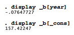
After any regression, Stata temporarily remembers coefficients and other details. Thus _b[varname] refers to the coefficient on independent variable varname. _b[_cons] refers to the coefficient on _cons (usually, the y-intercept).
Although predict makes it easy to calculate predicted values and residuals, we could have defined the same variables through a pair of generate statements using the _b[ ] coefficients. The resulting variables, named areahatl and arearesl below, have exactly the same properties as the predicted values and residuals from predict, but for certain purposes the generate approach gives users more flexibility.
. generate areahatl = _b[_cons] + _b[year]*year
. generate arearesl = area – areahatl
. summarize area*
Source: Hamilton Lawrence C. (2012), Statistics with STATA: Version 12, Cengage Learning; 8th edition.
3 Oct 2022
3 Oct 2022
28 Sep 2022
3 Oct 2022
24 Sep 2022
28 Sep 2022