Random Intercepts and Slopes by using Stata

In Figure 13.2 we saw that, overall, the percentage of Bush votes tended to decline as population density increased. Our random-intercept model in the previous section accepted this generalization, while allowing intercepts to vary across regions. But what if the slope of the votes-density relationship also varies across regions? A quick look at scatterplots for each region (Figure 13.4) gives us grounds to suspect that it does.

. graph twoway scatter bush logdens, msymbol(Oh)

|| lfit bush logdens, lwidth(medthick)

|| , xlabel(-1(1)4, grid) ytitle(“Percent vote for GW Bush”)

by(cendiv, legend(off) note(“”))

Bush votes decline most steeply with rising density in the Pacific and W North Central regions, but there appears to be little relationship in the E North Central, and even a positive effect in the E South Central. The negative fixed-effect coefficient on logdens in our previous model was averaging these downward, flat and upward trends together.

A mixed model including random slopes (u _jj) on predictor x_j, and random intercepts (u_0j) for each of j groups could have the general form

To estimate such a model, we add the predictor variable logdens to the mixed-effect part of the xtmixed command.

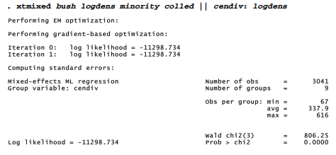
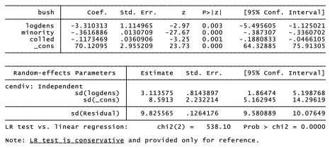
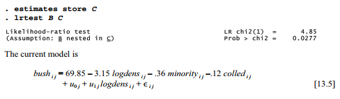
As usual, the random effects are not directly estimated. Instead, the xtmixed table gives estimates of their standard deviations. The standard deviation for coefficients on log density is 3.11 — almost four standard errors (.81) from zero — suggesting that there exists significant division-to-division variation in the slope coefficients. A more definitive likelihood-ratio test will support this inference. To perform this test, we quietly re-estimate the intercept-only model, store those estimates as A (an arbitrary name) then re-estimate the intercept-and-slope model, store those estimates as B, and finally perform a likelihood-ratio test for whether B fits significantly better than A. In this example it does (p~ .0000), so we conclude that adding random slopes brought significant improvement.

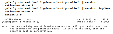
This lrtest output warns that it “assumes the null hypothesis is not on the boundary of the parameter space,” otherwise the reported test is conservative. A note at the bottom of the previous xtmixed output also stated that its likelihood-ratio test is conservative. Both notes refer to the same statistical issue. Variance cannot be less than zero, so a null hypothesis stating a variance equals zero does lie on the boundary of the parameter space. In this situation the reported likelihood-ratio test probability represents an upper bound (“conservative”) for the actual probability. xtmixed detects the situation automatically, but it is not practical for lrtest to do so, hence the “If …” wording from the latter.

The previous model assumes that random intercept and slopes are uncorrelated, equivalent to adding a cov(independent) option specifying the covariance structure. Other possibilities include cov(unstructured), which would allow for a distinct, nonzero covariance between the random effects.

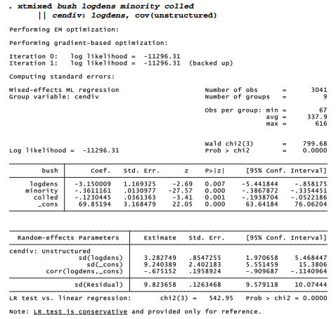
The estimated correlation between the random slope on logdens and the random intercept is -.675, more than three standard errors from zero. A likelihood-ratio test agrees that allowing for this correlation results in significant (p = .0277) improvement over our previous model.

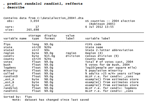
So what are the slopes relating votes to density for each census division? Again, we can obtain values for the random effects (here named randintl and randslol) through predict. Our dataset by now contains several new variables.

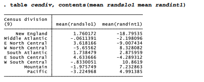
The random slope coefficients range from -5.66 for counties in the W North Central division, to +4.63 in the E South Central.

To clarify the relationship between votes and population density we could rearrange equation [13.5], combining the fixed and random slopes on logdens,

In other words, the slope for each census division equals the fixed-effect slope for the whole sample, plus the random-effect slope for that division. Among Pacific counties, for instance, the combined slope is -3.15 – 3.22 = -6.37. The nine combined slopes are calculated and graphed in Figure 13.5.

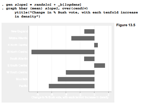
Figure 13.5 shows how the rural-urban gradient in voting behavior worked differently in different places. In counties of the W North Central, Pacific and Mountain regions, the percent voting for Bush declined most steeply as population density increased. In the E North Central and E South Central it went the other way — Bush votes increased slightly as density increased. The combined slopes in Figure 13.5 generally resemble those in the separate scatterplots of Figure 13.4, but do not match them exactly because our combined slopes (equation [13.6] or Figure 13.5) also adjust for the effects of minority and college-educated populations. In the next section we consider whether those effects, too, might have random components.

Source: Hamilton Lawrence C. (2012), Statistics with STATA: Version 12, Cengage Learning; 8th edition.