Problem 11.3: Mixed MANOVA with SPSS

There might be times when you want to find out if there are differences between groups as well as within subjects; this can be answered with Mixed MANOVA.

We have created a new dataset to use for this problem (MixedMANOVAdata).

• Retrieve MixedMANOVAdata.sav.

Let’s answer the following question:

• Is there a difference between participants in the intervention group (group 1) and participants in the control group (group 2) in the amount of change that occurs over time in scores on two different outcome

measures?

We will not check the assumptions of linearity, multivariate normality, or homogeneity of variance-covariance matrices because MANOVA is robust against these assumptions when the sample sizes are equal. If our sample sizes had not been approximately equal, we would need to check these assumptions.

• Analyze → General Linear Model → Repeated Measures (see 11.3).
• Delete the factor 1 from the Within-Subject Factor Name box and replace it with the name time, our name for the repeated-measures independent variable that SPSS will generate.
• Type 2 in the Number of Levels
• Click on Add.
• In the Measure Name box, type dv1.
• Click on Add.
• In the Measure Name box, type dv2.
• Click on Add. The window should look like 11.3.

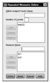
Fig. 11.3. Repeated measures define factor(s).

• Click on Define, which changes the screen to a new menu box (see Fig.10.4 in Chapter 10 if you need help).

• Now while holding down the “shift” key, click on outcome 1 pretest, outcome 1 posttest, outcome 2 pretest, and outcome 2 posttest. Click on the arrow to move these over to the Within-Subjects Variables
• Highlight group and then click on the arrow to move it over to the Between-Subjects Factor(s) box.
• Click on Plots. The Repeated Measures: Profile Plots window will open.
• Highlight time and then click on the arrow to move it to the Horizontal Axis
• Highlight group and then click on the arrow to move it to the Separate Lines
• Click on Add. This will move the variables down to the Plots

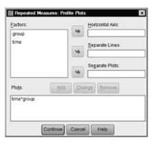
Fig. 11.4. Repeated measures: Profile plots.

• Click on Continue.
• Click on Options (see 10.6 in Chapter 10 if you need help).
• Click on Descriptive Statistics, Estimates of effect size, Observed power, and Homogeneity tests.
• Click on Continue, then on OK.

Compare your syntax and output with Output 11.3.

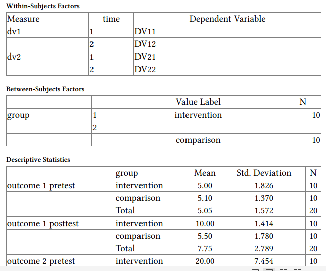
Output 11.3: Repeated Measures MANOVA Using the General Linear Model

GLMDV11 DV12 DV21 DV22 BY group /WSFACTOR = time 2 Polynomial /MEASURE = dv1 dv2

/METHOD = SSTYPE(3)

/PLOT = PROFILE(time*group)

/PRINT = DESCRIPTIVE ETASQ OPOWER HOMOGENEITY

/CRITERIA = ALPHA(.05)

/WSDESIGN = time

/DESIGN = group.

General Linear Model

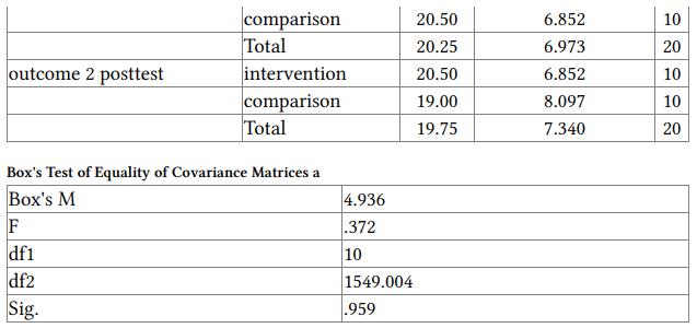
Tests the null hypothesis that the observed covariance matrices of the dependent variables are equal across groups.

a Design: Intercept+group Within Subjects Design: time

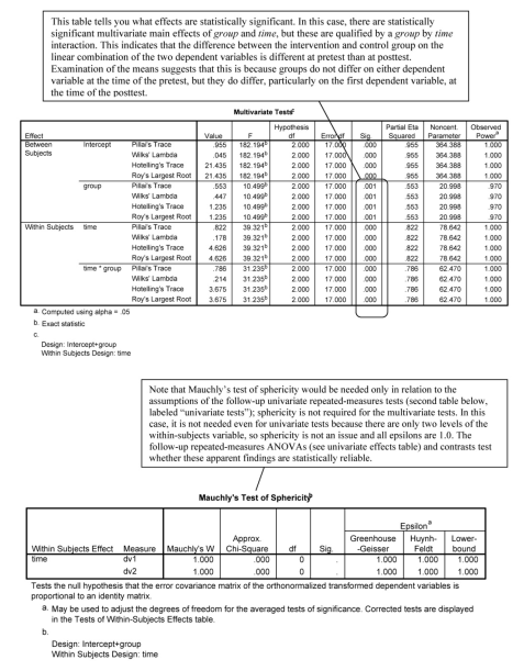
Interpretation of Output 11.3

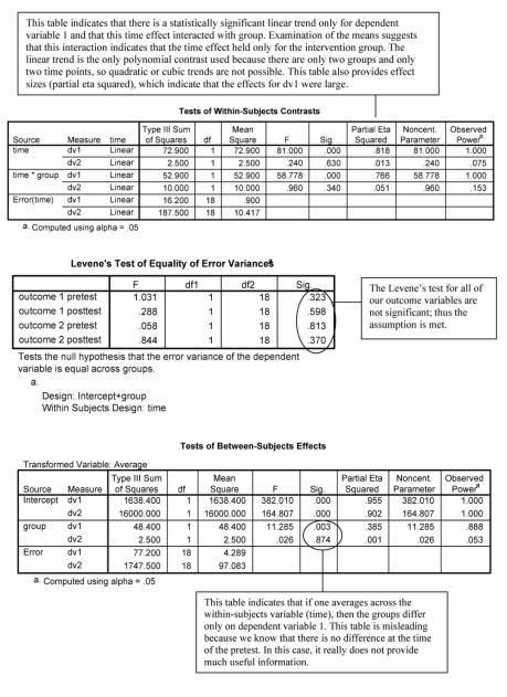
This example illustrates the utility of the doubly multivariate analysis for testing a pretest-posttest design with intervention and control groups. We see from these results not only that the intervention seemed successful when both outcome measures were taken together but also that the effect was statistically significant only for one of the dependent variables, when each was considered separately. Sphericity was not an issue in this case because there were only two levels of the within-subjects variable. If one creates difference scores by subtracting each person’s score on the dependent variable at one level of the within-subjects variable from the same dependent variable at each other level of the within-subjects variable, then sphericity exists if the variances of the resulting difference scores are all equal. Because there are only two levels of the within-subjects variable, there is only one set of difference scores, so sphericity has to exist, which is desirable. If we had had more than two levels of the within-subjects variable, then we would have needed to be concerned about the sphericity assumption when examining the univariate results. If epsilons did not approach 1.0, then we would have used the Huynh-Feldt or Greenhouse- Geisser test results, which use an estimate of epsilon to correct the degrees of freedom. Levene’s Test for homogeneity of variances was not significant, therefore this assumption was met.

Example of How to Write About Problem 11.3

Results

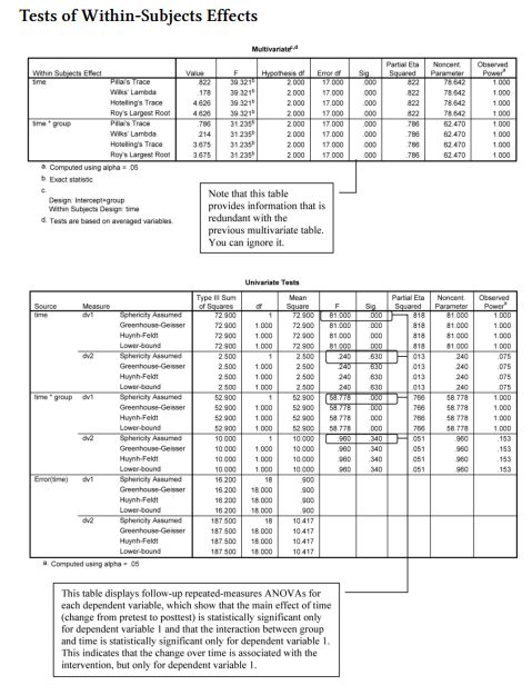
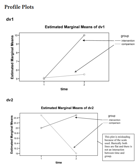
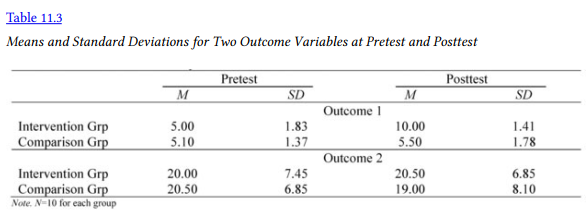
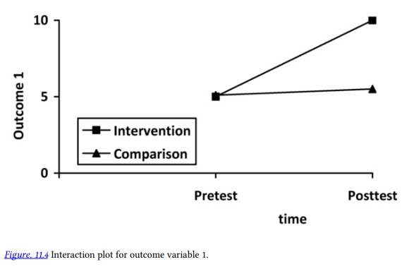
A doubly multivariate analysis was conducted to assess if there was a difference between participants in the intervention group and participants in the control group in the amount of change in their scores on the two outcome measures. (The sample sizes were equal across the groups; therefore, the assumptions were considered to be met.) Statistically significant multivariate effects were found for the main effects of group, F(2, 17) = 10.50, p = .001 and time F(2, 17) = 39.3, p < .001, as well as for the interaction between group and time, F(2, 17) = 31.20, p < .001. This interaction effect indicates that the difference between the intervention and control group on the linear combination of the two dependent variables is different at pretest than it is at posttest. Table 11.3 presents the means and standard deviations on the two variables. Examination of the means shows why the interaction is statistically significant; the groups do not differ much on either dependent variable at the time of the pretest, but they do differ, particularly on the first dependent variable, at the time of the posttest. Follow-up ANOVAs reveal that the statistically significant change from pretest to posttest was statistically significant only for the first outcome variable, F(1, 18) = 81.00, p < .001, and that the change in the first outcome variable was different for the two groups, F(1, 18) = 58.78, p < .001. Figure 11.4 displays the interaction effect for this variable. Examination of the means in Table 11.3 suggests that the change in the first outcome variable only held for the intervention group.

Source: Leech Nancy L. (2014), IBM SPSS for Intermediate Statistics, Routledge; 5th edition;

download Datasets and Materials.