Problem 9.1: Factorial (Two-Way) ANOVA with SPSS

We would use a t test or one-way ANOVA to examine differences between two or more groups (comprising the levels of one independent variable or factor) on a continuous dependent variable. These designs, in which there is only one independent variable and it is a discrete or categorical variable, are called single­factor designs. In this problem, we will compare groups formed by combining two independent variables. The appropriate statistic for this type of problem is called a two-factor, two-way, or factorial ANOVA. One can also have factorial ANOVAs in which there are more than two independent variables. If there are three independent variables, one would have a three-factor or threeway ANOVA. It is unusual, but possible, to have more than three factors as well. Factorial ANOVA is used when there are two or more independent variables (each with a few categories or values) and a between-groups design.

9.1 Are there differences in math achievement for people varying on math grades and/or father’s education revised, and is there a significant interaction between math grades and father’s education on math achievement? (Another way to ask this latter question: Do the “effects” of math grades on math achievement vary depending on level of father’s education revised?)

Follow these commands:

• Analyze → General Linear Model → Univariate.
• Move math achievement to the Dependent Variable
• Move the first independent variable, math grades, to the Fixed Factor(s) box and then move the second independent variable, father’s educ revised (not father’s education), to the Fixed Factor(s) box (see 9.1).

Now that we know the variables we will be dealing with, let’s determine our options.

Fig.9.1.GLM: Univariate.

• Click on Plots and move faedRevis to the Horizontal Axis and mathgr to the Separate Lines box in 9.2. This “profile plot” will help you picture the interaction (or absence of interaction) between your two independent variables. Note, the plots will be easier to interpret if you put father’s educ revised with its three values on the horizontal axis and create separate lines for the variable (math grades) that has two levels.
• Then press Add. You will see that mathgr and faedRevis have moved to the Plots window as shown at the bottom of 9.2.
• Click on Continue to get back 9.1.

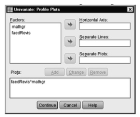
Fig.9.2.Univariate: Profile plots.

Select Options and check Descriptive statistics, Estimates of effect size, Observed power, and Homogeneity tests in Fig. 9.3.

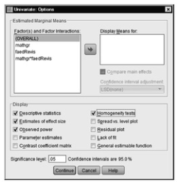
Fig.9.3.Univariate: Options.

• Click on Continue. This will take you back to 9.1.
• Click on OK. Compare your output with Output 9.1.

Output 9.1: GLM General Factorial (Two-Way) ANOVA

UNIANOVA mathach BY mathgr faedRevis /METHOD = SSTYPE(3) /INTERCEPT = INCLUDE

/PLOT = PROFILE(faedRevis*mathgr)

/PRINT = OPOWER ETASQ HOMOGENEITY DESCRIPTIVE

/CRITERIA = ALPHA(.05)

/DESIGN = mathgr faedRevis mathgr*faedRevis.

Univariate Analysis of Variance

Profile Plots

Interpretation of Output 9.1

The GLM Univariate program allows you to print the means and counts, measures of effect size (partial eta²), and the plot of the interaction, which is helpful in interpreting it. The first table in Output 9.1 shows the two levels of math grades (0 and 1), with 43 participants indicating “less A-B” (low math grades) and 30 reporting “most A-B” (high grades). Father’s education revised had three levels (low, medium, and high education) with 38 participants reporting HS grad or less, 16 indicating some college, and 19 with a BS or more. The second table, Descriptive Statistics, shows the cell and marginal (total) means; both are very important for interpreting the ANOVA table and explaining the results of the test for the interaction.

The second table is Levene’s Test of Equality of Error Variances, which tests the homogeneity of variances. It is important to check whether Levene’s test is significant; if it is significant (p < .05) the variances are different, and thus this assumption is violated. If it is not significant (p > .05), then the assumption is met. Whether this assumption has been met is important to remember when we do post hoc tests.

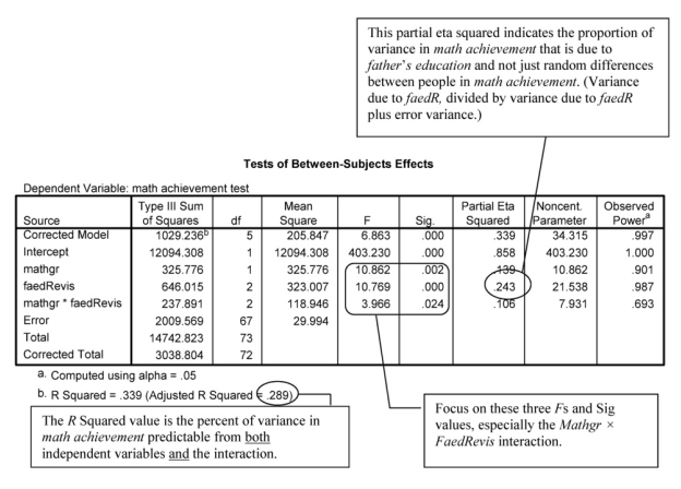
The ANOVA table, called Tests of BetweenSubjects Effects, is the key table. Note that the word “effect” in the title of the table can be misleading because this study was not a randomized experiment. Thus, you should not report that the differences in the dependent variable were caused by the independent variable. Usually you will ignore the information about the corrected model and intercept and skip down to the interaction F (mathgr*faedRevis). It is important to look at the interaction first because it may change the interpretation of the separate “main effects” of each independent variable.

In this case, the interaction is statistically significant, F(2,67) = 3.97, p = .024. This means that the “effect” of math grades on math achievement depends on which father’s education level is being considered. If you find a significant interaction, you should examine the profile plots of cell means to visualize the differential effects. If there is a significant interaction, the lines on the profile plot will not be parallel. In this case, the plot indicates that math achievement is relatively low for both groups of students whose fathers had relatively low education (high school grad or less). However, for students whose fathers have a high education level (BS or more), differences in math grades seem to have a large “effect” on math achievement. This interpretation, based on a visual inspection of the plots, needs to be checked with inferential statistics. When the interaction is statistically significant, you should analyze the “simple effects” (differences between means for one variable at each particular level of the other variable). We will illustrate two methods for statistically analyzing the simple effects in Problem 9.2.

Now examine the main effects of math grades and of father’s education revised. Note that both are statistically significant, but because the interaction is significant this is somewhat misleading. The plots show that the effect of math grades does not seem to hold true for those whose fathers had the least education. Note also the callout boxes about the adjusted R squared and partial eta squared. Eta, the correlation ratio, is used when the independent variable is nominal and the dependent variable (math achievement in this problem) is scale. Eta is an indicator of the proportion of variance that is due to between-groups differences. Partial eta squared is the ratio of the variance associated with a particular between-groups “effect” to the sum of that same number (variance associated with that “effect”) and error variance. So it is a measure of reliable variance in the DV (math achievement in this case) that is associated with a particular between-groups “effect.” Adjusted R² refers to the multiple correlation coefficient, squared and adjusted for number of independent variables, N, and effect size. Like r², partial eta squared and R² indicate how much variance or variability in the dependent variable can be predicted; however, the multiple R² is used when there are several independent variables, and the r² is used when there is only one independent variable. In this problem, the partial eta² values for the three key Fs vary from .106 to .243 (you can take the square root of this to get partial eta, which in this case varies from

.325 to .493). Because partial eta and R, like r, are indexes of association, they can be used to interpret the effect size. However, the guidelines according to Cohen (1988) for eta and R are somewhat different (for eta: small = .10, medium = .24, and large = .37; for R: small = .10, medium =.36, and large = .51).

An important point to remember is that statistical significance depends heavily on the sample size so that with 1,000 subjects, a much lower F or r will be significant than if the sample is 10 or even 100. Statistical significance just tells you that you can be quite sure that there is at least a tiny relationship between the independent and dependent variables. Effect size measures, which are more independent of sample size, tell how strong the relationship is and, thus, give you some indication of its importance.

The Observed Power for math grades was .90, and for father’s education revised it was .99. These indicate extremely high power, which means we might find statistically significant results even with small effect sizes. For these two factors this was not a problem because the effect sizes were large (partial etas = .373 and .493). Observed power for the interaction of math grades and father’s education revised was .69. Because it is less than .80, there was relatively low power. But, because the effect size for the interaction was close to large (partial eta = .326), we had enough power to detect this difference.

How to write the results for Problem 9.1 is included after the interpretation box for Problem 9.2.

Source: Leech Nancy L. (2014), IBM SPSS for Intermediate Statistics, Routledge; 5th edition;

download Datasets and Materials.