We have described, in the interpretation of Output 9.1, how to visually inspect and interpret the Profile Plots when there is a statistically significant interaction.
In Problems 9.2b and 9.2c we will illustrate two ways to test the simple effects statistically.
In the interpretation of Output 9.1, we indicated that you should examine the interaction F first. If it is statistically significant, it provides important information and means that the results of the main effects may be misleading. Figure 9.4 is a decision tree that illustrates this point and guides the analysis in this section. It shows two ways to examine the simple effects when you have a significant interaction. You would use either contrasts or post hoc tests, not both.
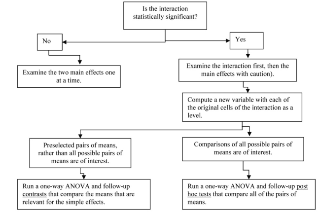
Fig. 9.4. Steps in analyzing a two-way factorial ANOVA.
9.2. Which simple effects of math grades (at each level of father’s education revised) are statistically significant?
9.2a. Computation of the New Cellcode Variable
To analyze the simple effects, we first need to compute a new variable with each of the original cells as a level. To do this, do the following commands.
- Select Transform → Compute Variable… You will see the Compute Variable window, Fig. 9.5.
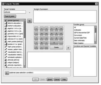
Fig.9.5.Compute variable window.
- Under Target Variable, type cellcode. This is the name of the new variable you will compute.
- Click on Type and Label. You will see the Compute Variable: Type and Label window ( 9.6).
- Type six new cell codes in the label box.
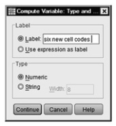
Fig.9.6.Compute variable: Type and label.
- Click on Continue. You will see the Compute Variable window ( 9.5) again.
- In the Numeric Expression box, type the number 1. This will be the first value or level for the new variable.
- Next, click on the If… button in 9.5 to produce Fig. 9.7.
- Select Include if case satisfies condition.
- Type mathgr = 0 & faedRevis = 1 in the window. You are telling SPSS to compute level 1 of the new variable, cellcode, so that it combines the first level of math grades (0) and the first level of father’s education revised (1) (see 9.7).
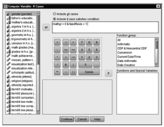
Fig. 9.7. Compute variable: If cases.
- Click on Continue to return to 9.5.
- Click on OK. If you look at your Data View or Variable View screen, you will see a new variable called cellcode. In the Data View screen, you should also notice that several of the cases now show a value of 1. Those are the cases where the original variables of math grades and father’s education revised met the requirements you just computed.
You will need to repeat this process for the other five levels of this new variable. We will walk you through the process once more.
- Select Transforms→ Compute Variable to see the Compute Variable window (see Fig. 9.5).
- Ensure that cellcode is still in the target variable box.
- Delete the 1 on the Numeric Expression
- Type 2 in the Numeric Expression
- Click on the .. button.
- Ensure that Include if case satisfies condition is selected.
- Type mathgr=1 & faedRevis=1 in the box. You are now telling SPSS to use the other (higher) level of math grades with the first level of father’s education revised.
- Click on Continue.
- Click on OK.
- SPSS will ask you if you want to change the existing variable. Click on OK. This means that you want to add this second level to the cellcode If you look at the Data View screen, you will notice that some of the cases now indicate a value of 2.
- Complete the above steps for the remaining four levels: Level 3 of cellcode: mathgr = 0 & faedRevis = 2; Level 4: mathgr = 1 & faedRevis = 2; Level 5: mathgr = 0 & faedRevis = 3; and Level 6: mathgr = 1 & faedRevis = 3.
To simplify the output and help you remember what levels you have created, you should add value labels to the cellcode variable as we have done in Output 9.2b. See Appendix A if you don’t know how to do this, and see Output 9.2b for the labels we used.
Output 9.2a
IF (mathgr = 0 & faedRevis = 1 ) cellcode = 1.
EXECUTE.
IF (mathgr = 1 & faedRevis = 1 ) cellcode = 2.
EXECUTE.
IF (mathgr = 0 & faedRevis = 2 ) cellcode = 3.
EXECUTE.
IF (mathgr = 1 & faedRevis = 2 ) cellcode = 4.
EXECUTE.
IF (mathgr = 0 & faedRevis = 3) cellcode = 5.
EXECUTE.
IF (mathgr = 1 & faedRevis = 3) cellcode = 6.
EXECUTE.
Next, you will use this new variable, cellcode, to examine the statistical significance of differences among certain of the six cells. This will help us to interpret the simple effects that we discussed above. We will demonstrate two types of follow-up tests (Post Hoc tests and Contrasts), but you should choose the most appropriate, not both. Remember, Post Hoc tests are appropriate when the researcher does not have a clear idea of which levels of the independent variable she/he wishes to compare or wants to compare all pairs of levels. Therefore, with Post Hoc tests all possible combinations will be compared. Contrasts compare a limited number of preselected pairs of means rather than all possible pairs of means. We will use the GLM univariate program to do post hocs in Problem 9.2b, but we could have used the Oneway program as we did in 9.2c.
9.2b. Computation of Post Hoc Tests
- Select Analyze → General Linear Model → Univariate. (This will produce 9.1.)
- Click on Reset.
- Move math achievement to the Dependent (variable) box.
- Move six new cell codes to the Fixed Factor(s)
- Click on Post Hoc… The Univariate: Post Hoc Multiple Comparisons for Observed Means window (not shown) will appear.
- Highlight cellcode in the Factors Click on the arrow to move it into the Post Hoc Tests for: box.
- Click on the Games-Howell post hoc test under Equal Variances Not Assumed because the Levene’s test for homogeneity was significant in Output 9.1. (If Levene’s test for homogeneity had not been significant, we could use the Tukey post hoc test here.)
- Click on Continue to get 9.1. Select Options to get Fig. 9.3.
- Check Descriptive statistics, Estimates of effect size, and Observed power. (Don’t check homogeneity tests; we already know that it is significant.)
- Click on Continue and OK.
Output 9.2b.
UNIANOVA mathach BY cellcode /METHOD = SSTYPE(3) /INTERCEPT = INCLUDE /POSTHOC = cellcode (GH)
/PRINT = DESCRIPTIVE ETASQ OPOWER
/CRITERIA = ALPHA(.05)
/DESIGN = cellcode.
Univariate Analysis of Variance
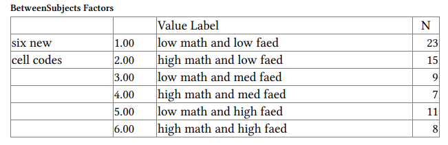
BetweenSubjects Factors
Descriptive Statistics
Post Hoc Tests
six new cell codes
Interpretation of Output 9.2b
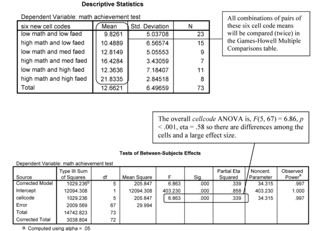
The second table is Descriptive Statistics showing the six new cell code means computed in Output 9.2a. The Tests of BetweenSubjects Effects table provides an overall or omnibus ANOVA (circled) that indicates there are significant differences among the six cellcode means. However, we are almost always more interested in the comparisons of pairs or other subsets of the means. Post hoc multiple comparisons allow you to test all combinations of pairs of means or at least more combinations of interest than are allowed using contrasts.
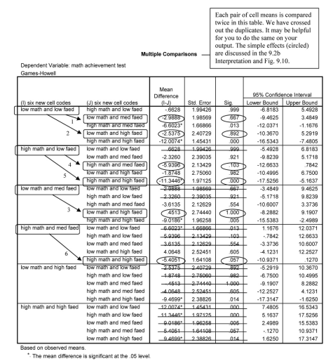
The Multiple Comparisons table is very complex. It includes comparisons of all possible combinations of pairs of cellcode means, twice. We have crossed out duplicates to simplify the table some. Even then there are 15 paired comparisons, and some are more meaningful than others. One useful set of comparisons is to test the difference between high and low math grades at each level of father’ s education. We have done this in Output 9.2c and Fig. 9.11 with contrasts. Similar comparisons are made in this table. Can you find them?
Another set of meaningful comparisons is identified by the circles in the Multiple Comparisons table and by Fig. 9.10. These post hoc comparisons show that there are no significant differences between any of the three pairs of means for the low math grades line in Fig. 9.10. The p values for comparisons 1, 2, and 3 are .667, .892, and 1.00, respectively. Can you see them in the figure and table?
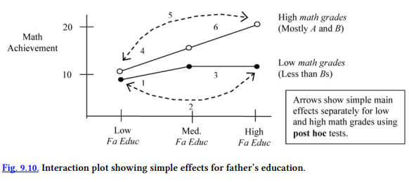
In regard to students who had high math grades (the top line), there was not a significant difference between the low and medium father’s education groups (comparison 4, p = .103) or between the medium and high father’s education groups (6, p = .057). However, there was a difference for the high math grades students between those with father’s who were HS grads or less (low) and those with a B.S. or more (high); this is comparison 5 and p < .001.
Example of How to Write About Problems 9.1 and 9.2 With Post Hoc Tests
Results
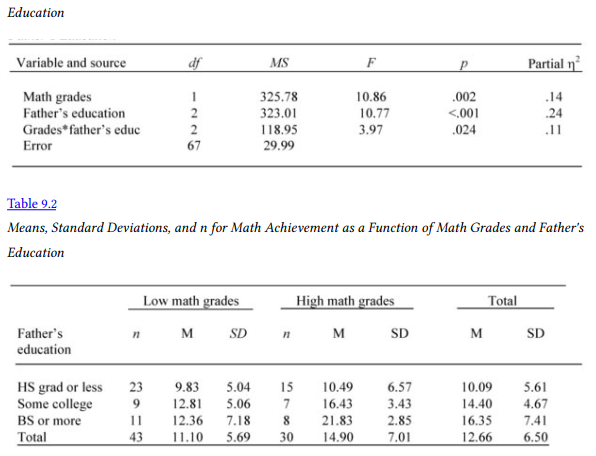
Table 9.1 shows that there was a significant interaction between the effects of math grades and father’s education on math achievement, F(2,67) = 3.97, p = .024, partial eta2 = .11. (The assumptions of independent observations was met, and assumptions of homogeneity of variances and normal distributions of the dependent variable for each group were checked. The assumption of homogeneity of variances was violated; thus, results should be viewed with caution. The assumption of normal distributions of the dependent variable for each group was not violated.) Table 9.2 shows the number of subjects, the mean, and standard deviation of math achievement for each cell. Games-Howell post hoc tests revealed that, of students with low math grades, level of father’s education did not seem to be associated with differences in math achievement. In contrast, for those who had mostly A and Bs in math, high father education was associated with statistically significantly higher math achievement than low father education (p < .001, d = 2.02). This effect size is considered large according to the literature.
9.2c. Computation of Contrasts
If you have preselected a limited number of comparisons between means, the appropriate follow-up test is Contrasts. Note that the maximum number of contrasts that you can do is limited in an SPSS run to the number of levels of the independent variable minus one, so that the number of contrasts will not exceed the number of degrees of freedom. To do Contrasts follow the steps below.
- Select Analyze→ Compare Means→ One Way ANOVA… You will see the One Way ANOVA (See Fig. 9.8.)
- Move math achievement into the Dependent List: box by clicking on the top arrow
- Move six new cell codes into the Factor: box by clicking on the bottom arrow button.
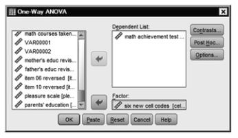
Fig.9.8.One-Way ANOVA.
Now, we will compute Contrasts. In this case, we want to compare the math achievement of high versus low math grade students at each of the three levels of father’s education. This is done by telling SPSS specific cell means to contrast. For example, if we want to compare only the first and second means while ignoring the other four means, we would write a contrast statement as follows 1 -1 0 0 0 0. This can be done with the SPSS syntax or using the point and click method as shown below.
- Click on the .. button to see Fig. 9.9.
- Enter 1 in the Coefficients: window.
- Then click on Add, which will move the 1 to the larger window.
- Next enter -1 and press Add; enter 0, press Add; enter another 0, press Add.
- Enter a third 0, press Add; enter a fourth 0. Fig 9.9 is how the window should look just before you press Add the final time. This compares the math achievement scores of students with low versus high math grades if their fathers have the lowest level of education.
- Now press Next so that the 9.9 says Contrast 2 of 2.
- Now enter the following coefficients as you did for the first contrast: 0 0 1 -1 0 0. Be sure to press Add after you enter each number. This compares the math achievement scores of students with low versus high grades if their fathers have the middle level of education.
- Press Next and enter the following Coefficients for Contrast 3 of 3: 0 0 0 0 1 -1. This compares the math achievement scores of students with low versus high grades if their fathers have the highest level of education.
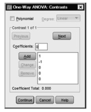
Fig.9.9.One-Way ANOVA: Contrasts.
Thus, what we have done with the above instructions is simple effects, first comparing students with high and low math grades who have fathers with less than a high school education. Second, we have compared students with high and low math grades who have fathers with some college. Finally, we have compared students with high and low math grades who have fathers with a B.S. or more. Look back at how we computed the cellcode variable (or the syntax and Descriptives in Output 9.2c) to see why this is true. Note that in cases like this it might be easier to type the syntax, which is part of the reason many experienced SPSS users prefer to use syntax. However, you must type the syntax exactly correctly or the program will not run.
- Click on Continue.
- Click on Options.
- Click on Descriptive and Homogeneity of variance test.
- Click on Continue.
- Click on OK.
Output 9.2c: Contrasts for Comparing New Cell Means
ONEWAY mathach BY cellcode /CONTRAST= 1 -1 0 0 0 0
/CONTRAST= 0 0 1 -1 0 0
/CONTRAST= 0 0 0 0 1 -1
/STATISTICS DESCRIPTIVES HOMOGENEITY
/MISSING ANALYSIS.
Oneway
Interpretation of Output 9.2c
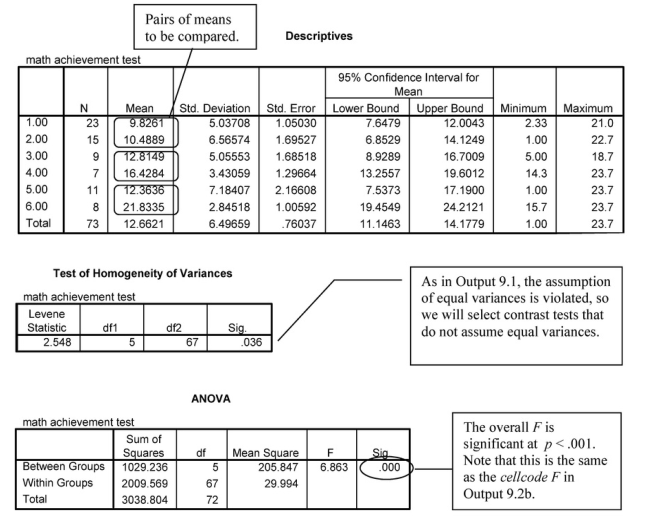
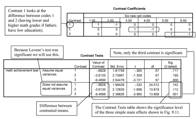
This output is the result of doing the bottom left-hand step, shown in Fig. 9.4, for interpreting a statistically significant interaction. Using Output 9.2c, we can examine three main simple effects statistically. The first table, Descriptives, provides the means of the six new cell code groups that will be compared, two at a time, as shown in the Contrast Coefficients table. The second table is Levene’s test for the assumption that the variances are equal or homogeneous. In this case, the Levene’s test is significant, so the assumption is violated and the variances cannot be assumed to be equal. The third table is the ANOVA table. Again, the overall F(5,67) = 6.86 is significant (p < .001), which indicates that there are significant differences somewhere. The Contrast Tests table helps us identify which simple effects were statistically significant. We will focus on one set of simple effects in our interpretation, the ones based on t tests that do not assume equal variances. Note that we have circled three Sigs. (the significance level or p). These correspond to the three simple effects shown with arrows in our drawing of the interaction plot (Fig. 9.11). For example, the left-hand arrow (and the first contrast) compares math achievement scores for both high and low math grades of students whose fathers have a relatively low education level.

The contrasts confirm statistically what we thought from visual inspection of the profile plot in Output 9.1. As you can see in Fig. 9.11 and the circled parts of the Contrast Tests table, there is not a significant difference (p = .742) in math achievement between students with high and low math grades when their father’s education is low. Likewise, the difference between students with high and low math grades when their father’s education is medium (some college), although bigger (3.61 points), is not statistically significant (p = .112). However, when father’s education is high, students with high (mostly As and Bs) math grades do much better (9.47 points) on the achievement test than those with low grades (p = .001). Thus, math achievement depends both on students’ math grades and their father’s education. It would also be possible to examine the simple effects for high and low math grades separately (the two lines) as we did in the interpretation for 9.2b, but it is usually not necessary to do both types of simple effects to understand the interaction.
Example of How to Write About Problems 9.1 and 9.2 With Contrasts
Results
Table 9.3 shows that there was a significant interaction between the effects of math grades and father’s education on math achievement, F(2,67) = 3.97, p = .024, partial eta2 = .11. (The assumption of independent observations was met, and assumptions of homogeneity of variances and normal distributions of the dependent variable for each group were checked. The assumption of homogeneity of variances was violated; thus, results should be viewed with caution. The assumption of normal distributions of the dependent variable for each group was not violated.) Table 9.4 shows the number of subjects, the mean, and standard deviation of math achievement for each cell. Simple effects contrast analyses revealed that, of students with highly educated fathers, those who had mostly A and B grades had higher math achievement than did students who had lower grades, t(13.86) = -3.97, p = .001). Simple effects at the other levels of father education were not significant, indicating that for students whose fathers were less educated, students with higher and lower math grades had similar math achievement scores.
Source: Leech Nancy L. (2014), IBM SPSS for Intermediate Statistics, Routledge; 5th edition;
download Datasets and Materials.
27 Mar 2023
29 Mar 2023
27 Mar 2023
31 Mar 2023
27 Mar 2023
16 Sep 2022