Random Experiments, Counting Rules, and Assigning Probabilities

In discussing probability, we deal with experiments that have the following characteristics:

1. The experimental outcomes are well defined, and in many cases can even be listed prior to conducting the experiment.
2. On any single repetition or trial of the experiment, one and only one of the possible experimental outcomes will occur.
3. The experimental outcome that occurs on any trial is determined solely by chance. We refer to these types of experiments as random experiments.

To illustrate the key features associated with a random experiment, consider the process of tossing a coin. Referring to one face of the coin as the head and to the other face as the tail, after tossing the coin the upward face will be either a head or a tail. Thus, there are two possible experimental outcomes: head or tail. On an any single repetition or trial of this experiment, only one of the two possible experimental out­comes will occur; in other words, each time we toss the coin we will either observe a head or a tail. And, the outcome that occurs on any trial is determined solely by chance or random variability. As a result, the process of tossing a coin is considered a random experiment.

By specifying all the possible experimental outcomes, we identify the sample space for a random experiment.

An experimental outcome is also called a sample point to identify it as an element of the sample space.

Consider the random experiment of tossing a coin. If we let S denote the sample space, we can use the following notation to describe the sample space.

S   = {Head, Tail}

The random experiment of tossing a coin has two experimental outcomes (sample points). As an illustration of a random experiment with more than two experimental outcomes, consider the process of rolling a die. The possible experimental outcomes, defined as the number of dots appearing on the face of the die, are the six sample points in the sample space for this random experiment,

S = {1, 2, 3, 4, 5, 6}

1. Counting Rules, Combinations, and Permutations

Being able to identify and count the experimental outcomes is a necessary step in assigning probabilities. We now discuss three useful counting rules.

Multiple-Step Experiments The first counting rule applies to multiple-step experiments.

Consider the experiment of tossing two coins. Let the experimental outcomes be defined in terms of the pattern of heads and tails appearing on the upward faces of the two coins. How many experimental outcomes are possible for this experiment? The experiment of tossing two coins can be thought of as a two-step experiment in which step 1 is the tossing of the first coin and step 2 is the tossing of the second coin. If we use H to denote a head and T to denote a tail, (H, H ) indicates the experimental outcome with a head on the first coin and a head on the second coin. Continuing this notation, we can describe the sample space (S) for this coin-tossing experiment as follows:

S = {(H, H ), (H, T ), (T, H ), (T, T )}

Thus, we see that four experimental outcomes are possible. In this case, we can easily list all the experimental outcomes.

The counting rule for multiple-step experiments makes it possible to determine the number of experimental outcomes without listing them.

Counting rule for multiple-step experiments

If an experiment can be described as a sequence of k steps with n possible outcomes on the first step, n₂ possible outcomes on the second step, and so on, then the total number of experimental outcomes is given by (n₁) (n₂) . . . (n_k).

Viewing the experiment of tossing two coins as a sequence of first tossing one coin (n₁ = 2) and then tossing the other coin (n₂ = 2), we can see from the counting rule that (2)(2) = 4 distinct experimental outcomes are possible. As shown, they are S = {(H, H), (H, T), (T, H), (T, T)}. The number of experimental outcomes in an experiment involving tossing six coins is (2)(2)(2)(2)(2)(2) = 64.

A tree diagram is a graphical representation that helps in visualizing a multiple-step experiment. Figure 4.2 shows a tree diagram for the experiment of tossing two coins. The sequence of steps moves from left to right through the tree. Step 1 corresponds to tossing the first coin, and step 2 corresponds to tossing the second coin. For each step, the two possible outcomes are head or tail. Note that for each possible outcome at step 1 two branches correspond to the two possible outcomes at step 2. Each of the points on the right end of the tree corresponds to an experimental outcome. Each path through the tree from the leftmost node to one of the nodes at the right side of the tree corre­sponds to a unique sequence of outcomes.

Let us now see how the counting rule for multiple-step experiments can be used in the analysis of a capacity expansion project for the Kentucky Power & Light Company (KP&L). KP&L is starting a project designed to increase the generating capacity of one of its plants in northern Kentucky. The project is divided into two sequential stages or steps: stage 1 (design) and stage 2 (construction). Even though each stage will be scheduled and controlled as closely as possible, management cannot predict beforehand the exact time required to complete each stage of the project. An analysis of similar construction projects revealed possible completion times for the design stage of 2, 3, or 4 months and possible completion times for the construction stage of 6, 7, or 8 months. In addition, because of the critical need for additional electrical power, management set a goal of 10 months for the completion of the entire project.

Because this project has three possible completion times for the design stage (step 1) and three possible completion times for the construction stage (step 2), the counting rule for multiple-step experiments can be applied here to determine a total of (3)(3) = 9 experi­mental outcomes. To describe the experimental outcomes, we use a two-number notation; for instance, (2, 6) indicates that the design stage is completed in 2 months and the con­struction stage is completed in 6 months. This experimental outcome results in a total of 2 + 6 = 8 months to complete the entire project. Table 4.1 summarizes the nine experi­mental outcomes for the KP&L problem. The tree diagram in Figure 4.3 shows how the nine outcomes (sample points) occur.

The counting rule and tree diagram help the project manager identify the exper­imental outcomes and determine the possible project completion times. From the information in Figure 4.3, we see that the project will be completed in 8 to 12 months, with six of the nine experimental outcomes providing the desired completion time of 10 months or less. Even though identifying the experimental outcomes may be helpful, we need to consider how probability values can be assigned to the experimental out­comes before making an assessment of the probability that the project will be com­pleted within the desired 10 months.

Combinations A second useful counting rule allows one to count the number of experimental outcomes when the experiment involves selecting n objects from a set of N objects. It is called the counting rule for combinations.

As an illustration of the counting rule for combinations, consider a quality control procedure in which an inspector randomly selects two of five parts to test for defects. In a group of five parts, how many combinations of two parts can be selected? The counting rule in equation (4.1) shows that with N = 5 and n = 2, we have

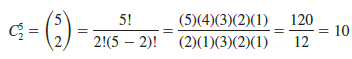
Thus, 10 outcomes are possible for the experiment of randomly selecting two parts from a group of five. If we label the five parts as A, B, C, D, and E, the 10 combina­tions or experimental outcomes can be identified as AB, AC, AD, AE, BC, BD, BE, CD, CE, and DE.

As another example, consider that the Florida Lotto lottery system uses the random selection of 6 integers from a group of 53 to determine the weekly winner. The counting rule for combinations, equation (4.1), can be used to determine the number of ways 6 different integers can be selected from a group of 53.

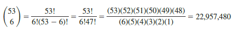
The counting rule for combinations tells us that almost 23 million experimental outcomes are possible in the lottery drawing. An individual who buys a lottery ticket has 1 chance in 22,957,480 of winning.

Permutations A third counting rule that is sometimes useful is the counting rule for permutations. It allows one to compute the number of experimental outcomes when n objects are to be selected from a set of N objects where the order of selection is important. The same n objects selected in a different order are considered a different experimental outcome.

The counting rule for permutations closely relates to the one for combinations; however, an experiment results in more permutations than combinations for the same number of objects because every selection of n objects can be ordered in n! different ways.

As an example, consider again the quality control process in which an inspector selects two of five parts to inspect for defects. How many permutations may be selected? The counting rule in equation (4.2) shows that with N = 5 and n = 2, we have

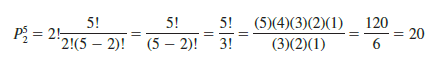
Thus, 20 outcomes are possible for the experiment of randomly selecting two parts from a group of five when the order of selection must be taken into account. If we label the parts A, B, C, D, and E, the 20 permutations are AB, BA, AC, CA, AD, DA, AE, EA, BC, CB, BD, DB, BE, EB, CD, DC, CE, EC, DE, and ED.

2. Assigning Probabilities

Now let us see how probabilities can be assigned to experimental outcomes. The three ap­proaches most frequently used are the classical, relative frequency, and subjective methods. Regardless of the method used, two basic requirements for assigning probabilities must be met.

The classical method of assigning probabilities is appropriate when all the experimen­tal outcomes are equally likely. If n experimental outcomes are possible, a probability of 1/n is assigned to each experimental outcome. When using this approach, the two basic requirements for assigning probabilities are automatically satisfied.

For an example, consider the experiment of tossing a fair coin; the two experimental outcomes—head and tail—are equally likely. Because one of the two equally likely out­comes is a head, the probability of observing a head is 1/2, or .50. Similarly, the proba­bility of observing a tail is also 1/2, or .50.

As another example, consider the experiment of rolling a die. It would seem reasonable to conclude that the six possible outcomes are equally likely, and hence each outcome is assigned a probability of 1/6. If P(1) denotes the probability that one dot appears on the upward face of the die, then P(1) = 1/6. Similarly, P(2) = 1/6, P(3) = 1/6, P(4) = 1/6,

P(5) = 1/6, and P(6) = 1/6. Note that these probabilities satisfy the two basic requirements of equations (4.3) and (4.4) because each of the probabilities is greater than or equal to zero and they sum to 1.0.

The relative frequency method of assigning probabilities is appropriate when data are available to estimate the proportion of the time the experimental outcome will occur if the experiment is repeated a large number of times. As an example, consider a study of waiting times in the X-ray department for a local hospital. A clerk recorded the number of patients waiting for service at 9:00 a.m. on 20 successive days and obtained the following results.

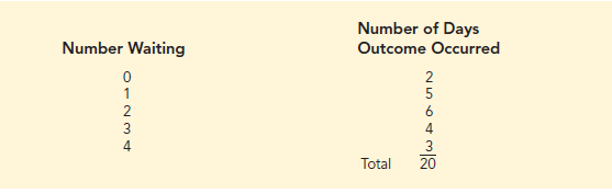
These data show that on 2 of the 20 days, zero patients were waiting for service; on 5 of the days, one patient was waiting for service; and so on. Using the relative frequency method, we would assign a probability of 2/20 = .10 to the experimental outcome of zero patients waiting for service, 5/20 = .25 to the experimental outcome of one patient waiting, 6/20 = .30 to two patients waiting, 4/20 = .20 to three patients waiting, and 3/20 = .15 to four patients waiting. As with the classical method, using the relative frequency method automatically satisfies the two basic requirements of equations (4.3) and (4.4).

The subjective method of assigning probabilities is most appropriate when one cannot realistically assume that the experimental outcomes are equally likely and when little rel­evant data are available. When the subjective method is used to assign probabilities to the experimental outcomes, we may use any information available, such as our experience or intuition. After considering all available information, a probability value that expresses our degree of belief (on a scale from 0 to 1) that the experimental outcome will occur is spec­ified. Because subjective probability expresses a person’s degree of belief, it is personal. Using the subjective method, different people can be expected to assign different proba­bilities to the same experimental outcome.

The subjective method requires extra care to ensure that the two basic requirements of equations (4.3) and (4.4) are satisfied. Regardless of a person’s degree of belief, the proba­bility value assigned to each experimental outcome must be between 0 and 1, inclusive, and the sum of all the probabilities for the experimental outcomes must equal 1.0.

Consider the case in which Tom and Judy Elsbernd make an offer to purchase a house. Two outcomes are possible:

E₁ = their offer is accepted

E₂ = their offer is rejected

Judy believes that the probability their offer will be accepted is .8; thus, Judy would set P(E₁) = .8 and P(E₂) = .2. Tom, however, believes that the probability that their offer will be accepted is .6; hence, Tom would set P(E₁) = .6 and P(E₂) = .4. Note that Tom’s proba­bility estimate for E₁ reflects a greater pessimism that their offer will be accepted.

Both Judy and Tom assigned probabilities that satisfy the two basic requirements. The fact that their probability estimates are different emphasizes the personal nature of the subjective method.

Even in business situations where either the classical or the relative frequency approach can be applied, managers may want to provide subjective probability estimates. In such cases, the best probability estimates often are obtained by combining the estimates from the classical or relative frequency approach with subjective probability estimates.

3. Probabilities for the KP&L Project

To perform further analysis on the KP&L project, we must develop probabilities for each of the nine experimental outcomes listed in Table 4.1. On the basis of experience and judgment, management concluded that the experimental outcomes were not equally likely. Hence, the classical method of assigning probabilities could not be used. Management then decided to conduct a study of the completion times for similar projects undertaken by KP&L over the past three years. The results of a study of 40 similar projects are summa­rized in Table 4.2.

After reviewing the results of the study, management decided to employ the relative frequency method of assigning probabilities. Management could have provided subjective probability estimates but felt that the current project was quite similar to the 40 previous projects. Thus, the relative frequency method was judged best.

In using the data in Table 4.2 to compute probabilities, we note that outcome (2, 6)—stage 1 completed in 2 months and stage 2 completed in 6 months—occurred six times in the 40 projects. We can use the relative frequency method to assign a probability of 6/40 = .15 to this outcome. Similarly, outcome (2, 7) also occurred in six of the 40 projects, providing a 6/40 = .15 probability. Continuing in this manner, we obtain the probability assignments for the sample points of the KP&L project shown in Table 4.3. Note that P(2, 6) represents the probability of the sample point (2, 6), P(2, 7) represents the probability of the sample point (2, 7), and so on.

Source:  Anderson David R., Sweeney Dennis J., Williams Thomas A. (2019), Statistics for Business & Economics, Cengage Learning; 14th edition.