Thus far we have considered the completely randomized experimental design. Recall that to test for a difference among treatment means, we computed an F value by using the ratio
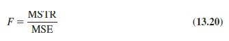
A problem can arise whenever differences due to extraneous factors (ones not considered in the experiment) cause the MSE term in this ratio to become large. In such cases, the F value in equation (13.20) can become small, signaling no difference among treatment means when in fact such a difference exists.
In this section we present an experimental design known as a randomized block design. Its purpose is to control some of the extraneous sources of variation by removing such variation from the MSE term. This design tends to provide a better estimate of the true error variance and leads to a more powerful hypothesis test in terms of the ability to detect differences among treatment means. To illustrate, let us consider a stress study for air traffic controllers.
1. Air Traffic Controller Stress Test
A study measuring the fatigue and stress of air traffic controllers resulted in proposals for modification and redesign of the controller’s workstation. After consideration of several designs for the workstation, three specific alternatives are selected as having the best potential for reducing controller stress. The key question is: To what extent do the three alternatives differ in terms of their effect on controller stress? To answer this question, we need to design an experiment that will provide measurements of air traffic controller stress under each alternative.
In a completely randomized design, a random sample of controllers would be assigned to each workstation alternative. However, controllers are believed to differ substantially in their ability to handle stressful situations. What is high stress to one controller might be only moderate or even low stress to another. Hence, when considering the within-group source of variation (MSE), we must realize that this variation includes both random error and error due to individual controller differences. In fact, managers expected controller variability to be a major contributor to the MSE term.
One way to separate the effect of the individual differences is to use a randomized block design. Such a design will identify the variability stemming from individual controller differences and remove it from the MSE term. The randomized block design calls for a single sample of controllers. Each controller in the sample is tested with each of the three workstation alternatives. In experimental design terminology, the workstation is the factor of interest and the controllers are the blocks. The three treatments or populations associated with the workstation factor correspond to the three workstation alternatives. For simplicity, we refer to the workstation alternatives as system A, system B, and system C.
The randomized aspect of the randomized block design is the random order in which the treatments (systems) are assigned to the controllers. If every controller were to test the three systems in the same order, any observed difference in systems might be due to the order of the test rather than to true differences in the systems.

To provide the necessary data, the three workstation alternatives were installed at the Cleveland Control Center in Oberlin, Ohio. Six controllers were selected at random and assigned to operate each of the systems. A follow-up interview and a medical examination of each controller participating in the study provided a measure of the stress for each controller on each system. The data are reported in Table 13.5.
Table 13.6 is a summary of the stress data collected. In this table we include column totals (treatments) and row totals (blocks) as well as some sample means that will be helpful in making the sum of squares computations for the ANOVA procedure. Because lower stress values are viewed as better, the sample data seem to favor system B with its mean stress rating of 13. However, the usual question remains: Do the sample results justify the conclusion that the population mean stress levels for the three systems differ? That is, are the differences statistically significant? An analysis of variance computation similar to the one performed for the completely randomized design can be used to answer this statistical question.

2. ANOVA Procedure
The ANOVA procedure for the randomized block design requires us to partition the sum of squares total (SST) into three groups: sum of squares due to treatments (SSTR), sum of squares due to blocks (SSBL), and sum of squares due to error (SSE). The formula for this partitioning follows.
SST = SSTR + SSBL + SSE (13.21)
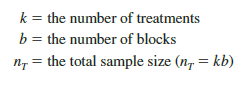
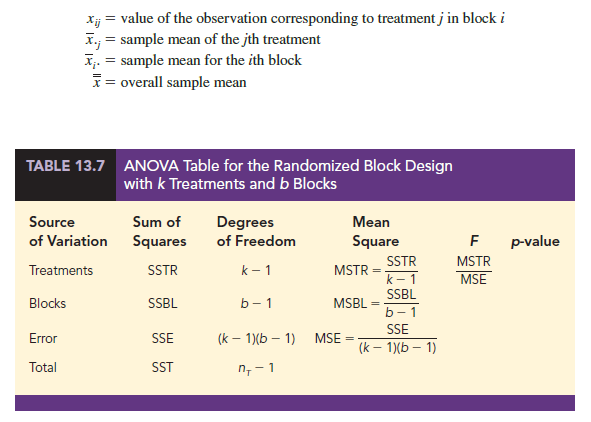
This sum of squares partition is summarized in the ANOVA table for the randomized block design as shown in Table 13.7. The notation used in the table is
Note that the ANOVA table also shows how the nT – 1 total degrees of freedom are partitioned such that k – 1 degrees of freedom go to treatments, b – 1 go to blocks, and (k – 1)(b – 1) go to the error term. The mean square column shows the sum of squares divided by the degrees of freedom, and F = MSTR/MSE is the F ratio used to test for a significant difference among the treatment means. The primary contribution of the randomized block design is that by including blocks, we remove the individual controller differences from the MSE term and obtain a more powerful test for the stress differences in the three workstation alternatives.
3. Computations and Conclusions
To compute the F statistic needed to test for a difference among treatment means with a randomized block design, we need to compute MSTR and MSE. To calculate these two mean squares, we must first compute SSTR and SSE; in doing so, we will also compute SSBL and SST. To simplify the presentation, we perform the calculations in four steps. In addition to k, b, and nT as previously defined, the following notation is used.
Xj = value of the observation corresponding to treatment j in block i x.j = sample mean of the jth treatment Xi. = sample mean for the ith block X = overall sample mean
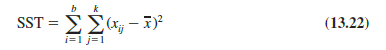
Step 1. Compute the total sum of squares (SST).
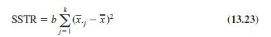
Step 2. Compute the sum of squares due to treatments (SSTR).
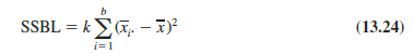
Step 3. Compute the sum of squares due to blocks (SSBL).
Step 4. Compute the sum of squares due to error (SSE).
SSE = SST – SSTR – SSBL (13.25)
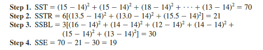
For the air traffic controller data in Table 13.6, these steps lead to the following sums of squares.
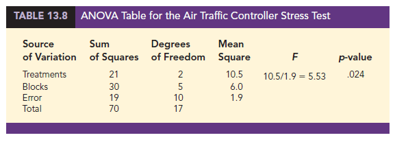
These sums of squares divided by their degrees of freedom provide the corresponding mean square values shown in Table 13.8.
Let us use a level of significance a = .05 to conduct the hypothesis test. The value of the test statistic is
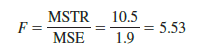
The numerator degrees of freedom is k – 1 = 3 – 1 = 2 and the denominator degrees of freedom is (k – 1)(b – 1) = (3 – 1)(6 – 1) = 10. Because we will only reject the null hypothesis for large values of the test statistic, the p-value is the area under the F distribution to the right of F = 5.53. From Table 4 of Appendix B we find that with the degrees of freedom 2 and 10, F = 5.53 is between F.025 = 5.46 and F.01 = 7.56. As a result, the area in the upper tail, or the p-value, is between .01 and .025. Alternatively, we can use statistical software to show that the exact p-value for F = 5.53 is .024. With p-value < a = .05, we reject the null hypothesis H0: m1 = m2 = m3 and conclude that the population mean stress levels differ for the three workstation alternatives.
Some general comments can be made about the randomized block design. The experimental design described in this section is a complete block design; the word “complete” indicates that each block is subjected to all k treatments. That is, all controllers (blocks) were tested with all three systems (treatments). Experimental designs in which some but not all treatments are applied to each block are referred to as incomplete block designs. A discussion of incomplete block designs is beyond the scope of this text.
Because each controller in the air traffic controller stress test was required to use all three systems, this approach guarantees a complete block design. In some cases, however, blocking is carried out with “similar” experimental units in each block. For example, assume that in a pretest of air traffic controllers, the population of controllers was divided into groups ranging from extremely high-stress individuals to extremely low-stress individuals. The blocking could still be accomplished by having three controllers from each of the stress classifications participate in the study. Each block would then consist of three controllers in the same stress group. The randomized aspect of the block design would be the random assignment of the three controllers in each block to the three systems.
Finally, note that the ANOVA table shown in Table 13.7 provides an F value to test for treatment effects but not for blocks. The reason is that the experiment was designed to test a single factor—workstation design. The blocking based on individual stress differences was conducted to remove such variation from the MSE term. However, the study was not designed to test specifically for individual differences in stress.
Some analysts compute F = MSB/MSE and use that statistic to test for significance of the blocks. Then they use the result as a guide to whether the same type of blocking would be desired in future experiments. However, if individual stress difference is to be a factor in the study, a different experimental design should be used. A test of significance on blocks should not be performed as a basis for a conclusion about a second factor.
Source: Anderson David R., Sweeney Dennis J., Williams Thomas A. (2019), Statistics for Business & Economics, Cengage Learning; 14th edition.
Good write-up, I’m regular visitor of one’s blog, maintain up the nice operate, and It’s going to be a regular visitor for a lengthy time.