Summarizing Data for Two Variables Using Graphical Displays

In the previous section we showed how a crosstabulation can be used to summarize the data for two variables and help reveal the relationship between the variables. In most cases, a graphical display is more useful for recognizing patterns and trends in the data.

In this section, we introduce a variety of graphical displays for exploring the relationships between two variables. Displaying data in creative ways can lead to powerful insights and al­low us to make “common-sense inferences” based on our ability to visually compare, contrast, and recognize patterns. We begin with a discussion of scatter diagrams and trendlines.

1. Scatter Diagram and Trendline

A scatter diagram is a graphical display of the relationship between two quantitative vari­ables, and a trendline is a line that provides an approximation of the relationship. As an illus­tration, consider the advertising/sales relationship for an electronics store in San Francisco.

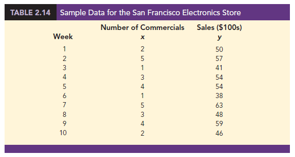
On 10 occasions during the past three months, the store used weekend television commercials to promote sales at its stores. The managers want to investigate whether a relationship exists between the number of commercials shown and sales at the store during the following week. Sample data for the 10 weeks with sales in hundreds of dollars are shown in Table 2.14.

Figure 2.8 shows the scatter diagram and the trendline^[1] for the data in Table 2.14. The num­ber of commercials (x) is shown on the horizontal axis and the sales (y) are shown on the verti­cal axis. For week 1, x = 2 and y = 50. A point with those coordinates is plotted on the scatter diagram. Similar points are plotted for the other nine weeks. Note that during two of the weeks one commercial was shown, during two of the weeks two commercials were shown, and so on.

The scatter diagram in Figure 2.8 indicates a positive relationship between the number of commercials and sales. Higher sales are associated with a higher number of commercials.

The relationship is not perfect in that all points are not on a straight line. However, the general pattern of the points and the trendline suggest that the overall relationship is positive.

Some general scatter diagram patterns and the types of relationships they suggest are shown in Figure 2.9. The top left panel depicts a positive relationship similar to the one for the number of commercials and sales example. In the top right panel, the scatter diagram shows no apparent relationship between the variables. The bottom panel depicts a negative relationship where y tends to decrease as x increases.

2. Side-by-Side and Stacked Bar Charts

In Section 2.1 we said that a bar chart is a graphical display for depicting categorical data summarized in a frequency, relative frequency, or percent frequency distribution. Side-by-side bar charts and stacked bar charts are extensions of basic bar charts that are used to display and compare two variables. By displaying two variables on the same chart, we may better understand the relationship between the variables.

A side-by-side bar chart is a graphical display for depicting multiple bar charts on the same display. To illustrate the construction of a side-by-side chart, recall the application involving the quality rating and meal price data for a sample of 300 restaurants located in the Los Angeles area. Quality rating is a categorical variable with rating categories of good, very good, and excellent. Meal price is a quantitative variable that ranges from $10 to $49. The crosstabulation displayed in Table 2.10 shows that the data for meal price were grouped into four classes: $10-19, $20-29, $30-39, and $40-49. We will use these classes to construct a side-by-side bar chart.

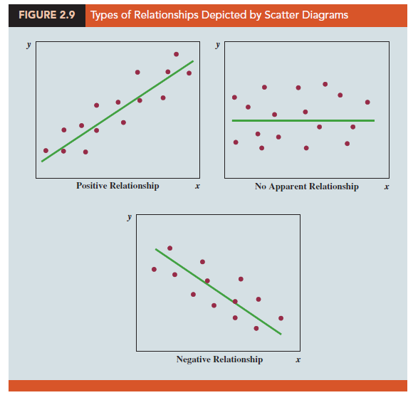
Figure 2.10 shows a side-by-side chart for the restaurant data. The color of each bar indicates the quality rating (light blue = good, medium blue = very good, and dark blue = excellent). Each bar is constructed by extending the bar to the point on the vertical axis that represents the frequency with which that quality rating occurred for each of the meal price categories. Placing each meal price category’s quality rating frequency adjacent to one another allows us to quickly determine how a particular meal price category is rated. We see that the lowest meal price category ($10-$19) received mostly good and very good ratings, but very few excellent ratings. The highest price category ($40-49), however, shows a much different result. This meal price category received mostly excellent ratings, some very good ratings, but no good ratings.

Figure 2.10 also provides a good sense of the relationship between meal price and quality rating. Notice that as the price increases (left to right), the height of the light blue bars decreases and the height of the dark blue bars generally increases. This indicates that as price increases, the quality rating tends to be better. The very good rating, as expected, tends to be more prominent in the middle price categories as indicated by the dominance of the middle bar in the moderate price ranges of the chart.

Stacked bar charts are another way to display and compare two variables on the same display. A stacked bar chart is a bar chart in which each bar is broken into rectangular segments of a different color showing the relative frequency of each class in a manner sim­ilar to a pie chart. To illustrate a stacked bar chart we will use the quality rating and meal price data summarized in the crosstabulation shown in Table 2.10.

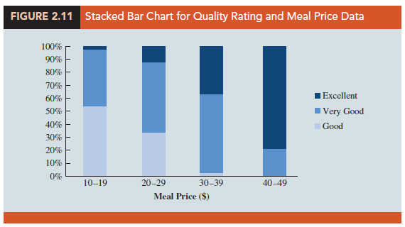
We can convert the frequency data in Table 2.10 into column percentages by dividing each element in a particular column by the total for that column. For instance, 42 of the 78 restaurants with a meal price in the $10-19 range had a good quality rating. In other words, (42/78)100 or 53.8% of the 78 restaurants had a good rating. Table 2.15 shows the column percentages for each meal price category. Using the data in Table 2.15 we constructed the stacked bar chart shown in Figure 2.11. Because the stacked bar chart is based on percent­ages, Figure 2.11 shows even more clearly than Figure 2.10 the relationship between the vari­ables. As we move from the low price category ($10-19) to the high price category ($40-49), the length of the light blue bars decreases and the length of the dark blue bars increases.

Source:  Anderson David R., Sweeney Dennis J., Williams Thomas A. (2019), Statistics for Business & Economics, Cengage Learning; 14th edition.