A probability distribution involving two random variables is called a bivariate probability distribution. In discussing bivariate probability distributions, it is useful to think of a bivariate experiment. Each outcome for a bivariate experiment consists of two values, one for each random variable. For example, consider the bivariate experiment of rolling a pair of dice. The outcome consists of two values, the number obtained with the first die and the number obtained with the second die. As another example, consider the experiment of observing the financial markets for a year and recording the percentage gain for a stock fund and a bond fund. Again, the experimental outcome provides a value for two random variables, the percent gain in the stock fund and the percent gain in the bond fund. When dealing with bivariate probability distributions, we are often interested in the relationship between the random variables. In this section, we introduce bivariate distributions and show how the covariance and correlation coefficient can be used as a measure of linear association between the random variables. We shall also see how bivariate probability distributions can be used to construct and analyze financial portfolios.
1. A Bivariate Empirical Discrete Probability Distribution
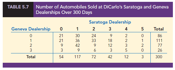
Recall that in Section 5.2 we developed an empirical discrete distribution for daily sales at the DiCarlo Motors automobile dealership in Saratoga, New York. DiCarlo has another dealership in Geneva, New York. Table 5.7 shows the number of cars sold at each of the dealerships over a 300-day period. The numbers in the bottom (total) row are the frequencies we used to develop an empirical probability distribution for daily sales at DiCarlo’s Saratoga dealership in Section 5.2. The numbers in the right-most (total) column are the frequencies of daily sales for the Geneva dealership. Entries in the body of the table give the number of days the Geneva dealership had a level of sales indicated by the row, when the Saratoga dealership had the level of sales indicated by the column. For example, the entry of 33 in the Geneva dealership row labeled 1 and the Saratoga column labeled 2 indicates that for 33 days out of the 300, the Geneva dealership sold 1 car and the Saratoga dealership sold 2 cars.
Suppose we consider the bivariate experiment of observing a day of operations at DiCarlo Motors and recording the number of cars sold. Let us define x = number of cars sold at the Geneva dealership and y = the number of cars sold at the Saratoga dealership. We can now divide all of the frequencies in Table 5.7 by the number of observations (300) to develop a bivariate empirical discrete probability distribution for automobile sales at the two DiCarlo dealerships. Table 5.8 shows this bivariate discrete probability distribution. The probabilities in the lower margin provide the marginal distribution for the DiCarlo Motors Saratoga dealership. The probabilities in the right margin provide the marginal distribution for the DiCarlo Motors Geneva dealership.
The probabilities in the body of the table provide the bivariate probability distribution for sales at both dealerships. Bivariate probabilities are often called joint probabilities. We see that the joint probability of selling 0 automobiles at Geneva and 1 automobile at Saratoga on a typical day is f(0, 1) = .1000, the joint probability of selling 1 automobile at Geneva and 4 automobiles at Saratoga on a typical day is .0067, and so on. Note that there is one bivariate probability for each experimental outcome. With 4 possible values for x and 6 possible values for y, there are 24 experimental outcomes and bivariate probabilities.
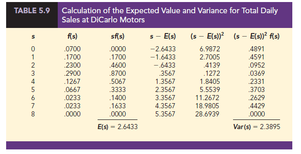
Suppose we would like to know the probability distribution for total sales at both DiCarlo dealerships and the expected value and variance of total sales. We can define 5 = x + y as total sales for DiCarlo Motors. Working with the bivariate probabilities in Table 5.8, we see that f(s = 0) = .0700, f(s = 1) = .0700 + .1000 = .1700, f(s = 2) = .0300 + .1200 + .0800 = .2300, and so on. We show the complete probability distribution for 5 = x + y along with the computation of the expected value and variance in Table 5.9. The expected value is E(s) = 2.6433 and the variance is Var(s) = 2.3895.
With bivariate probability distributions, we often want to know the relationship between the two random variables. The covariance and/or correlation coefficient are good measures of association between two random variables. The formula we will use for computing the covariance between two random variables x and y is given below.


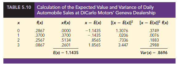
We have already computed Var(s) = Var(x + y) and, in Section 5.2, we computed Var (y). Now we need to compute Var(x) before we can use equation (5.6) to compute the covariance of x and y. Using the probability distribution for x (the right margin of Table 5.8), we compute E(x) and Var(x) in Table 5.10.
We can now use equation (5.6) to compute the covariance of the random variables x and y.
![]()
A covariance of .1350 indicates that daily sales at DiCarlo’s two dealerships have a positive relationship. To get a better sense of the strength of the relationship we can compute the correlation coefficient. The correlation coefficient for the two random variables x and y is given by equation (5.7).

From equation (5.7), we see that the correlation coefficient for two random variables is the covariance divided by the product of the standard deviations for the two random variables.
Let us compute the correlation coefficient between daily sales at the two DiCarlo dealerships. First we compute the standard deviations for sales at the Saratoga and Geneva dealerships by taking the square root of the variance.

Now we can compute the correlation coefficient as a measure of the linear association between the two random variables.

The correlation coefficient is a measure of the linear association between two variables. Values near +1 indicate a strong positive linear relationship; values near -1 indicate a strong negative linear relationship; and values near zero indicate a lack of a linear relationship. The correlation coefficient of .1295 indicates there is a weak positive relationship between the random variables representing daily sales at the two DiCarlo dealerships. If the correlation coefficient had equaled zero, we would have concluded that daily sales at the two dealerships were independent.
2. Financial Applications
Let us now see how what we have learned can be useful in constructing financial portfolios that provide a good balance of risk and return. A financial advisor is considering four possible economic scenarios for the coming year and has developed a probability distribution showing the percent return, x, for investing in a large-cap stock fund and the percent return, y, for investing in a long-term government bond fund given each of the scenarios. The bivariate probability distribution for x and y is shown in Table 5.11. Table 5.11 is simply a list with a separate row for each experimental outcome (economic scenario).

Each row contains the joint probability for the experimental outcome and a value for each random variable. Since there are only four joint probabilities, the tabular form used in Table 5.11 is simpler than the one we used for DiCarlo Motors where there were (4)(6) = 24 joint probabilities.
Using the formula in Section 5.3 for computing the expected value of a single random variable, we can compute the expected percent return for investing in the stock fund, E(x), and the expected percent return for investing in the bond fund, E(y).
E(x) = .10(-40) + .25(5) + .5(15) + .15(30) = 9.25
E(y) = .10(30) + .25(5) + .5(4) + .15(2) = 6.55
Using this information, we might conclude that investing in the stock fund is a better investment. It has a higher expected return, 9.25%. But, financial analysts recommend that investors also consider the risk associated with an investment. The standard deviation of percent return is often used as a measure of risk. To compute the standard deviation, we must first compute the variance. Using the formula in Section 5.3 for computing the variance of a single random variable, we can compute the variance of the percent returns for the stock and bond fund investments.
Var(x) = .1(—40 – 9.25)2 + .25(5 – 9.25)2 + .50(15 – 9.25)2 + .15(30 – 9.25)2 = 328.1875
Var(y) = .1(30 – 6.55)2 + .25(5 – 6.55)2 + .50(4 – 6.55)2 + .15(2 – 6.55)2 = 61.9475
The standard deviation of the return from an investment in the stock fund is σx = √328.1875 = 18.1159% and the standard deviation of the return from an investment in the bond fund is σy = √61.9475 = 7.8707%. So, we can conclude that investing in the bond fund is less risky. It has the smaller standard deviation. We have already seen that the stock fund offers a greater expected return, so if we want to choose between investing in either the stock fund or the bond fund it depends on our attitude toward risk and return. An aggressive investor might choose the stock fund because of the higher expected return; a conservative investor might choose the bond fund because of the lower risk. But, there are other options. What about the possibility of investing in a portfolio consisting of both an investment in the stock fund and an investment in the bond fund?
Suppose we would like to consider three alternatives: investing solely in the large- cap stock fund, investing solely in the long-term government bond fund, and splitting our funds equally between the stock fund and the bond fund (one-half in each). We have already computed the expected value and standard deviation for investing solely in the stock fund and the bond fund. Let us now evaluate the third alternative: constructing a portfolio by investing equal amounts in the large-cap stock fund and in the long-term government bond fund.
To evaluate this portfolio, we start by computing its expected return. We have previously defined x as the percent return from an investment in the stock fund and y as the percent return from an investment in the bond fund so the percent return for our portfolio is r = .5x + .5y. To find the expected return for a portfolio with one-half invested in the stock fund and one-half invested in the bond fund, we want to compute E(r) = E(.5x + .5y). The expression .5x + .5y is called a linear combination of the random variables x and y. Equation (5.8) provides an easy method for computing the expected value of a linear combination of the random variables x and y when we already know E(x) and E(y). In equation (5.8), a represents the coefficient of x and b represents the coefficient of y in the linear combination.
Since we have already computed E(x) = 9.25 and E(y) = 6.55, we can use equation (5.8) to compute the expected value of our portfolio.
E(.5x + .5y) = .5E(x) + .5E(y) = .5(9.25) + .5(6.55) = 7.9
We see that the expected return for investing in the portfolio is 7.9%. With $100 invested, we would expect a return of $100(.079) = $7.90; with $1000 invested we would expect a return of $1000(.079) = $79.00; and so on. But, what about the risk? As mentioned previously, financial analysts often use the standard deviation as a measure of risk.
Our portfolio is a linear combination of two random variables, so we need to be able to compute the variance and standard deviation of a linear combination of two random variables in order to assess the portfolio risk. When the covariance between two random variables is known, the formula given by equation (5.9) can be used to compute the variance of a linear combination of two random variables.

From equation (5.9), we see that both the variance of each random variable individually and the covariance between the random variables are needed to compute the variance of a linear combination of two random variables and hence the variance of our portfolio.
We have already computed the variance of each random variable individually:
Var(x) = 328.1875 and Var(y) = 61.9475.
Also, it can be shown that Var(x + y) = 119.46. So, using equation (5.6), the covariance of the random variables x and y is
![]()
A negative covariance between x and y, such as this, means that when x tends to be above its mean, y tends to be below its mean and vice versa.
We can now use equation (5.9) to compute the variance of return for our portfolio.
Var (.5x + .5y) = .52(328.1875) + .52(61.9475) + 2(.5)(.5)(-135.3375) = 29.865
The standard deviation of our portfolio is then given by ![]() .
.
This is our measure of risk for the portfolio consisting of investing 50% in the stock fund and 50% in the bond fund.
Perhaps we would now like to compare the three investment alternatives: investing solely in the stock fund, investing solely in the bond fund, or creating a portfolio by dividing our investment amount equally between the stock and bond funds. Table 5.12 shows the expected returns, variances, and standard deviations for each of the three alternatives.
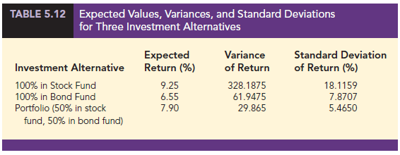
Which of these alternatives would you prefer? The expected return is highest for investing 100% in the stock fund, but the risk is also highest. The standard deviation is 18.1159%. Investing 100% in the bond fund has a lower expected return, but a significantly smaller risk. Investing 50% in the stock fund and 50% in the bond fund (the portfolio) has an expected return that is halfway between that of the stock fund alone and the bond fund alone. But note that it has less risk than investing 100% in either of the individual funds. Indeed, it has both a higher return and less risk (smaller standard deviation) than investing solely in the bond fund. So we would say that investing in the portfolio dominates the choice of investing solely in the bond fund.
Whether you would choose to invest in the stock fund or the portfolio depends on your attitude toward risk. The stock fund has a higher expected return. But the portfolio has significantly less risk and also provides a fairly good return. Many would choose it. It is the negative covariance between the stock and bond funds that has caused the portfolio risk to be so much smaller than the risk of investing solely in either of the individual funds.
The portfolio analysis we just performed was for investing 50% in the stock fund and the other 50% in the bond fund. How would you calculate the expected return and the variance for other portfolios? Equations (5.8) and (5.9) can be used to make these calculations easily.
Suppose we wish to create a portfolio by investing 25% in the stock fund and 75% in the bond fund? What are the expected value and variance of this portfolio? The percent return for this portfolio is r = .25x + .75y, so we can use equation (5.8) to get the expected value of this portfolio:
E(.25x + .75y) = .25E(x) + .75E(y) = .25(9.25) + .75(6.55) = 7.225
Likewise, we may calculate the variance of the portfolio using equation (5.9):
Var(.25x + .75y) = (.25)2Var(x) + (.75)2 Var(y) + 2(.25)(.75)sxy
= .0625(328.1875) + (.5625)(61.9475) + (.375)(—135.3375)
= 4.6056
![]()
Source: Anderson David R., Sweeney Dennis J., Williams Thomas A. (2019), Statistics for Business & Economics, Cengage Learning; 14th edition.
Im not likely to say what everyone else has already said, but I do want to comment on your knowledge of the topic. Youre truly well-informed.