The regression models above treat adolescent fertility, percent urban and other national characteristics as possible predictors of life expectancy, without necessarily asserting that they are its causes. One of those predictors, child mortality rate, has an obvious causal connection with life expectancy. But child mortality rates in turn are influenced by other national characteristics much as life expectancy is, complicating the causal picture. For example, if adolescent fertility rates affect child mortality and child mortality affects life expectancy, then adolescent fertility exerts an indirect effect on life expectancy whether or not it has a distinct effect directly. In causal terms, child mortality functions as an intervening or mediating variable.
Structural equation modeling provides a systematic way to analyze such indirect effects, along with other kinds of causal relationships. Its signature device is the path diagram, which visualizes our ideas about causal ordering and connections. The causal ordering of variables is critical. Structural equation modeling cannot prove causality, but rather assumes a particular causal structure. It then applies statistical techniques to fill in details, fine-tuning the
specification in some respects. We must rely on external knowledge or theory to specify the basic causal order, however. If that knowledge is shaky, then so are the analyses that follow. But sketching path diagrams is a useful step even when the ordering remains uncertain. Often the diagrams help to clarify fuzzy thinking, or better express our ideas.
Approaches based on structural equation modeling have become dominant in diverse areas of research. Since their early applications in the 1960s, structural equation models appealed to social scientists in particular because they promised to bridge worlds of theory and data. The models have been the focus of many books covering issues such as estimation, measurement models, error structures and reciprocal causation (e.g., Kline 2010; Skrondal and Rabe-Hesketh 2004). With version 12, Stata added its own structural equation modeling commands. To quote the Structural Equation Modeling Reference Manual:
“SEM is not just an estimation method for a particular model in the way that Stata’s regress and probit commands are, or even in the way that stcox and xtmixed are. SEM is a way of thinking, a way of writing, and a way of estimating.”
This section introduces Stata’s structural equation modeling command, sem, through a simple extension of our life expectancy regression. We have seen that life expectancy is predicted by other national characteristics. In the regression table below, the t statistics and beta weights or standardized regression coefficients (right-hand column) reveal that child mortality rate has by far the strongest effect.


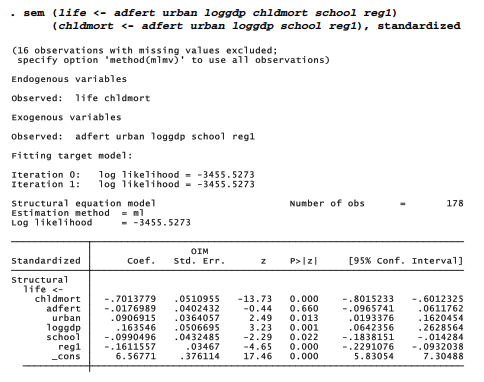
The standardized coefficients in this sem output equal the beta weights obtained by regress. Unlike regress, sem, reports standard errors for the standardized coefficients. These result in z statistics identical to the t statistics shown by regress but with slightly different probabilities because they are compared to standard normal rather than t distributions. The sem command’s parenthetical notation (life <- adfert urban loggdp chldmort school regl) specifies causal paths to life from adfert, urban etc.
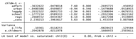
Child mortality, the strongest predictor of life expectancy, might be predicted from many of the same national characteristics. Adolescent fertility, which shows no significant effect on life expectancy in the regress or single-equation sem output above, turns out to be the strongest single predictor of child mortality.
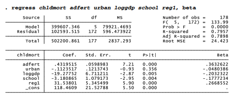
Figure 8.14 shows a path diagram in which child mortality appears as an intervening variable affected by adolescent fertility and other background characteristics, but is itself also a predictor of life expectancy. Conceptually, causality flows from left to right in this diagram. Indirect effects could follow any of the paths from background variables to chldmort, and then from chldmort to life. The boxes represent observed variables in this model; the topic of unobserved or latent variables is raised later, in Chapter 12.

The diagram in Figure 8.14 is drawn by a graphical user interface (GUI) called the SEM Builder. This GUI is invoked by typing the command
. sembuilder
or by menu choices
Statistics > SEM (structural equation modeling) > Model building and estimation
Type help sembuilder for information on how to get started. Basic elements in Figure 8.14 are the observed variables, first set in the diagram as empty boxes using the Add Observed Variable tool from the SEM Builder’s left-margin menu bar. Next the variable names are filled in by selecting each box with the Select tool, and filling in names from a pull-down Variable menu. An Add Path tool can draw in the paths connecting variables: click on the cause or exogenous variable, then drag the path arrow to connect with an effect or endogenous variable.
From the top menu bar, selecting Estimation > Estimate obtains coefficients and other statistics for the model. Figure 8.15 shows the default result of estimating Figure 8.14. Each path is associated with an unstandardized path or regression coefficient, such as .43 for the effect of adfert on chldmort (compare with the regression table above).
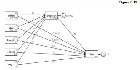
Within the box of each exogenous variable in Figure 8.15 we have the variable’s mean and its variance. Among the 178 nations used in this analysis, the mean adfert is approximately 54, and the variance is approximately 2.0e+03 = 2,000. The endogenous variable boxes contain their y- intercepts, such as 1.2e+02 = 120 for chldmort; again, compare with the previous regression results. Finally, Figure 8.15 gives residual variances associated with the error terms e1 (chldmort) and e2 (life).
A simplified version of this path diagram containing only standardized path coefficients and standardized residual variances appears in Figure 8.16. The simplification is obtained by making choices from the SEM Builder top menus:
Settings > Variables > All … > Results > Exogenous variables > None > OK
Settings > Variables > All … > Results > Endogenous variables > None > OK
Settings > Variables > Error … > Results > Error std. variance > OK
Settings > Connections > Paths > Results > Std. parameter > OK
Settings > Connections > All > Results > Result 1 > Format %3.2f > OK > OK
Estimation > Estimate > OK

. sem (life <- adfert urban loggdp chldmort school regl)
(chldmort <- adfert urban loggdp school regl), standardized
Indirect and total effects are easily calculated by hand. Indirect effects equal the product of coefficients along any series of causal paths that link one variable to another. Total effects equal the sum of all direct and indirect effects linking two variables. Reading standardized coefficients from Figure 8.16, adolescent fertility affects life expectancy as follows:
direct: -.02
indirect: .36 x (-.70) = – .25
total: -.02 – .25 = -.27
In other words, this model predicts that, other things being equal, a one standard deviation increase in adolescent fertility lowers the predicted life expectancy by .27 standard deviations through direct and indirect effects. The direct effect of adfert is near-zero, but it is causally important due to indirect effect through child mortality.
By similar calculations the influence of African location (standing in for troubles of that region not captured by other variables in the model) is more than double the direct effect of regl:
direct: -.16
indirect: .27 x (-.70) = -.19
total: -.16 – .19 = -.35
We return for a second look at structural equation modeling in the context of factor analysis, in Chapter 12.
Source: Hamilton Lawrence C. (2012), Statistics with STATA: Version 12, Cengage Learning; 8th edition.
28 Sep 2022
3 Oct 2022
23 Sep 2022
30 Sep 2022
23 Sep 2022
26 Sep 2022