Sampling in quantitative research

1. The concept of sampling

Let us take a very simple example to explain the concept of sampling. Suppose you want to estimate the average age of the students in your class. There are two ways of doing this. The first method is to contact all students in the class, find out their ages, add them up and then divide this by the number of students (the procedure for calculating an average). The second method is to select a few students from the class, ask them their ages, add them up and then divide by the number of students you have asked. From this you can make an estimate of the average age of the class. Similarly, suppose you want to find out the average income of families living in a city. Imagine the amount of effort and resources required to go to every family in the city to find out their income! You could instead select a few families to become the basis of your enquiry and then, from what you have found out from the few families, make an estimate of the aver­age income of families in the city. Similarly, election opinion polls can be used. These are based upon a very small group of people who are questioned about their voting preferences and, on the basis of these results, a prediction is made about the probable outcome of an election.

Sampling, therefore, is the process of selecting a few (a sample) from a bigger group (the sampling population) to become the basis for estimating or predicting the prevalence of an unknown piece of information, situation or outcome regarding the bigger group. A sample is a subgroup of the population you are interested in. See Figure 12.1.

This process of selecting a sample from the total population has advantages and disadvantages. The advantages are that it saves time as well as financial and human resources. However, the disad­vantage is that you do not find out the information about the population’s characteristics of interest to you but only estimate or predict them. Hence, the possibility of an error in your estimation exists.

Sampling, therefore, is a trade-off between certain benefits and disadvantages. While on the one hand you save time and resources, on the other hand you may compromise the level of accuracy in your findings. Through sampling you only make an estimate about the actual situation prevalent in the total population from which the sample is drawn. If you ascertain a piece of information from the total sampling population, and if your method of enquiry is correct, your findings should be reasonably accurate. However, if you select a sample and use this as the basis from which to estimate the situation in the total population, an error is pos­sible. Tolerance of this possibility of error is an important consideration in selecting a sample.

2. Sampling terminology

Let us, again, consider the examples used above where our main aims are to find out the average age of the class, the average income of the families living in the city and the likely election outcome for a particular state or country. Let us assume that you adopt the sampling method — that is, you select a few students, families or electorates to achieve these aims. In this process there are a number of aspects:

• The class, families living in the city or electorates from which you select you select your sample are called the population or study population, and are usually denoted by the letter N.
• The small group of students, families or electors from whom you collect the required information to estimate the average age of the class, average income or the election outcome is called the sample.
• The number of students, families or electors from whom you obtain the required information is called the sample size and is usually denoted by the letter n.
• The way you select students, families or electors is called the sampling design or sampling strategy.
• each student, family or elector that becomes the basis for selecting your sample is called the sampling unit or sampling element.
• a list identifying each student, family or elector in the study population is called the sampling frame. If all elements in a sampling population cannot be individually identified, you cannot have a sampling frame for that study population.
• Your findings based on the information obtained from your respondents (sample) are called sample statistics. your sample statistics become the basis of estimating the prevalence of the above characteristics in the study population.
• Your main aim is to find answers to your research questions in the study population, not in the sample you collected information from. From sample statistics we make an estimate of the answers to our research questions in the study population. The estimates arrived at from sample statistics are called population parameters or the population mean.

3. Principles of sampling

The theory of sampling is guided by three principles. To effectively explain these, we will take an extremely simple example. Suppose there are four individuals A, B, C and D. Further suppose that A is 18 years of age, B is 20, C is 23 and D is 25. As you know their ages, you can find out (calculate) their average age by simply adding 18 + 20 + 23 + 25 = 86 and dividing by 4. This gives the average (mean) age of A, B, C and D as 21.5 years.

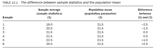
Now let us suppose that you want to select a sample of two individuals to make an estimate of the average age of the four individuals. To select an unbiased sample, we need to make sure that each unit has an equal and independent chance of selection in the sample. Randomisation is a process that enables you to achieve this. In order to achieve randomisa­tion we use the theory of probability in forming pairs which will provide us with six possible combinations of two: A and B; A and C; A and D; B and C; B and D; and C and D. Let us take each of these pairs to calculate the average age of the sample:

1. A + B = 18  + 20 = 38/2 = 19.0 years;
2. a + C = 18  + 23 = 41/2 = 20.5 years;
3. A + D = 18  + 25 = 43/2 = 21.5 years;
4. B + C = 20  + 23 = 43/2 = 21.5 years;
5. B + D = 20  + 25 = 45/2 = 22.5 years;
6. C + D = 23  + 25 = 48/2 = 24.0 years.

Notice that in most cases the average age calculated on the basis of these samples of two (sample statistics) is different. Now compare these sample statistics with the average of all four individuals — the population mean (population parameter) of 21.5 years. Out of a total of six possible sample combinations, only in the case of two is there no difference between the sample statistics and the population mean. Where there is a difference, this is attributed to the sample and is known as sampling error. Again, the size of the sampling error varies markedly. Let us consider the difference in the sample statistics and the population mean for each of the six samples (Table 12.1).

This analysis suggests a very important principle of sampling:

Principle 1 – in a majority of cases of sampling there will be a difference between the sample statistics and the true population mean, which is attributable to the selection of the units in the sample.

To understand the second principle, let us continue with the above example, but instead of a sample of two individuals we take a sample of three. There are four possible combinations of three that can be drawn:

1. A + B + C   = 18 + 20 +   23 = 61/3 =   33 years;
2. a + B + D   = 18 + 20 +   25 = 63/3 =   00 years;
3. A + C + D   = 18 + 23 +   25 = 66/3 =   00 years;
4. B + C + D   = 20 + 23 +   25 = 68/3 =   67 years.

Now, let us compare the difference between the sample statistics and the population mean (Table 12.2).

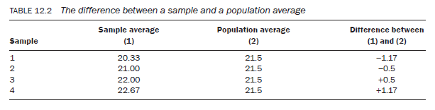
Compare the differences calculated in Table 12.1 and Table 12.2. In Table 12.1 the differ­ence between the sample statistics and the population mean lies between —2.5 and +2.5 years, whereas in the second it is between —1.17 and +1.17 years. The gap between the sample statistics and the population mean is reduced in Table 12.2. This reduction is attributed to the increase in the sample size. This, therefore, leads to the second principle:

Principle 2 — the greater the sample size, the more accurate the estimate of the true population mean.

The third principle of sampling is particularly important as a number of sampling strate­gies, such as stratified and cluster sampling, are based on it. To understand this principle, let us continue with the same example but use slightly different data. Suppose the ages of four individuals are markedly different: A = 18, B = 26, C = 32 and D = 40. In other words, we are visualising a population where the individuals with respect to age – the variable we are interested in — are markedly different.

Let us follow the same procedure, selecting samples of two individuals at a time and then three. If we work through the same procedures (described above) we will find that the differ­ence in the average age in the case of samples of two ranges between —7.00 and + 7.00 years and in the case of the sample of three ranges between —3.67 and +3.67. In both cases the range of the difference is greater than previously calculated. This is attributable to the greater difference in the ages of the four individuals — the sampling population. In other words, the sampling population is more heterogeneous (varied or diverse) in regard to age.

Principle 3 — the greater the difference in the variable under study in a population for a given sample size, the greater the difference between the sample statistics and the true population mean.

These principles are crucial to keep in mind when you are determining the sample size needed for a particular level of accuracy, and in selecting the sampling strategy best suited to your study.

4. Factors affecting the inferences drawn from a sample

The above principles suggest that two factors may influence the degree of certainty about the inferences drawn from a sample:

• The size of the sample – Findings based upon larger samples have more certainty than those based on smaller ones. As a rule, the larger the sample size, the more accurate the findings.
• The extent of variation in the sampling population – The greater the variation in the study population with respect to the characteristics under study, for a given sample size, the greater the uncertainty. (In technical terms, the greater the standard deviation, the higher the stand­ard error for a given sample size in your estimates.) If a population is homogeneous (uniform or similar) with respect to the characteristics under study, a small sample can provide a reason­ably good estimate, but if it is heterogeneous (dissimilar or diversified), you need to select a larger sample to obtain the same level of accuracy. Of course, if all the elements in a popula­tion are identical, then the selection of even one will provide an absolutely accurate estimate. As a rule, the higher the variation with respect to the characteristics under study in the study population, the greater the uncertainty for a given sample size.

5. Aims in selecting a sample

When you select a sample in quantitative studies you are primarily aiming to achieve maxi­mum precision in your estimates within a given sample size, and avoid bias in the selection of your sample.

Bias in the selection of a sample can occur if:

• sampling is done by a non-random method – that is, if the selection is consciously or uncon­sciously influenced by human choice;
• the sampling frame – list, index or other population records – which serves as the basis of selection, does not cover the sampling population accurately and completely;
• a section of a sampling population is impossible to find or refuses to co-operate.

6. Types of sampling

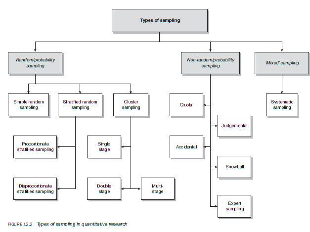
• random/probability sampling designs;
• non-random/non-probability sampling designs selecting a predetermined sample size;
• ‘mixed’ sampling design.

To understand these designs, we will discuss each type individually.

6.1. Random/probability sampling designs

For a design to be called random sampling or probability sampling, it is imperative that each element in the population has an equal and independent chance of selection in the sample. Equal implies that the probability of selection of each element in the popu­lation is the same; that is, the choice of an element in the sample is not influenced by other considerations such as personal preference. The concept of independence means that the choice of one element is not dependent upon the choice of another element in the sampling; that is, the selection or rejection of one element does not affect the inclu­sion or exclusion of another. To explain these concepts let us return to our example of the class.

Suppose there are 80 students in the class. Assume 20 of these refuse to participate in your study. You want the entire population of 80 students in your study but, as 20 refuse to par­ticipate, you can only use a sample of 60 students. The 20 students who refuse to participate could have strong feelings about the issues you wish to explore, but your findings will not reflect their opinions. Their exclusion from your study means that each of the 80 students does not have an equal chance of selection. Therefore, your sample does not represent the total class.

The same could apply to a community. In a community, in addition to the refusal to partici­pate, let us assume that you are unable to identify all the residents living in the community. If a significant proportion of people cannot be included in the sampling population because they either cannot be identified or refuse to participate, then any sample drawn will not give each element in the sampling population an equal chance of being selected in the sample. Hence, the sample will not be representative of the total community.

To understand the concept of an independent chance of selection, let us assume that there are five students in the class who are extremely close friends. If one of them is selected but refuses to participate because the other four are not chosen, and you are therefore forced to select either the five or none, then your sample will not be considered an independent sample since the selection of one is dependent upon the selection of others. The same could happen in the community where a small group says that either all of them or none of them will partici­pate in the study. In these situations where you are forced either to include or to exclude a part of the sampling population, the sample is not considered to be independent, and hence is not representative of the sampling population. However, if the number of refusals is fairly small, in practical terms, it should not make the sample non-representative. In practice there are always some people who do not want to participate in the study but you only need to worry if the number is significantly large.

A sample can only be considered a random/ probability sample (and therefore representative of the population under study) if both these conditions are met. Otherwise, bias can be intro­duced into the study.

There are two main advantages of random/probability samples:

• As they represent the total sampling population, the inferences drawn from such samples can be generalised to the total sampling population.
• Some statistical tests based upon the theory of probability can be applied only to data col­lected from random samples. Some of these tests are important for establishing conclusive correlations.

6.2. Methods of drawing a random sample

Of the methods that you can adopt to select a random sample the three most common are:

• The fishbowl draw – if your total population is small, an easy procedure is to number each element using separate slips of paper for each element, put all the slips into a box and then pick them out one by one without looking, until the number of slips selected equals the sample size you decided upon. This method is used in some lotteries.
• Computer program – there are a number of programs that can help you to select a random sample.
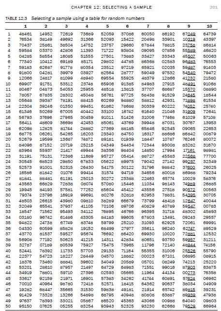
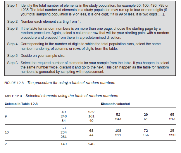
• A table of randomly generated numbers – most books on research methodology and statistics include a table of randomly generated numbers in their appendices (see, e.g., Table 12.3). You can select your sample using these tables according to the procedure described in Figure 12.3.

The procedure for selecting a sample using a table of random numbers is as follows:

Let us take an example to illustrate the use of Table 12.3 for random numbers. Let us assume that your sampling population consists of 256 individuals. Number each individual from 1 to 256. Randomly select the starting page, set of column (1 to 10) or row from the table and then identify three columns or rows of numbers.

Suppose you identify the ninth column of numbers and the last three digits of this column (underlined). Assume that you are selecting 10 per cent of the total population as your sample (25 elements). Let us go through the numbers underlined in the ninth set of columns. The first number is 049 which is below 256 (total population); hence, the 49th element becomes a part of your sample. The second number, 319, is more than the total elements in your population (256); hence, you cannot accept the 319th element in the sample. The same applies to the next element, 758, and indeed the next five elements, 589, 507, 483, 487 and 540. After 540 is 232, and as this number is within the sampling frame, it can be accepted as a part of the sample. Similarly, if you follow down the same three digits in the same column, you select 052, 029, 065, 246 and 161, before you come to the element 029 again. As the 29th element has already been selected, go to the next number, and so on until 25 elements have been chosen. Once you have reached the end of a column, you can either move to the next set of columns or randomly select another one in order to continue the process of selection. For example, the 25 elements shown in Table 12.4 are selected from the ninth, tenth and second columns of Table 12.3.

6.3. Sampling with or without replacement

Random sampling can be selected using two different systems:

1. sampling without replacement;
2. sampling with replacement.

Suppose you want to select a sample of 20 students out of a total of 80. The first student is selected out of the total class, and so the probability of selection for the first student is 1/80. When you select the second student there are only 79 left in the class and the probability of selection for the second student is not 1/80 but 1/79. The probability of selecting the next student is 1/78. By the time you select the 20th student, the probability of his/her selection is 1/61. This type of sampling is called sampling without replacement. But this is contrary to our basic definition of randomisation; that is, each element has an equal and independent chance of selection. In the second system, called sampling with replacement, the selected element is replaced in the sampling population and if it is selected again, it is discarded and the next one is selected. If the sampling population is fairly large, the probability of selecting the same element twice is fairly remote.

6.4. Specific random/probability sampling designs

There are three commonly used types of random sampling design.

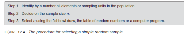
• Simple random sampling (SRS) – The most commonly used method of selecting a probability sample. In line with the definition of randomisation, whereby each element in the population is given an equal and independent chance of selection, a simple random sample is selected by the procedure presented in Figure 12.4.

To illustrate, let us again take our example of the class. There are 80 students in the class, and so the first step is to identify each student by a number from 1 to 80. Suppose you decide to select a sample of 20 using the simple random sampling technique. Use the fishbowl draw, the table for random numbers or a computer program to select the 20 students. These 20 students become the basis of your enquiry.

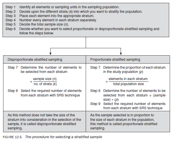
• Stratified random sampling – As discussed, the accuracy of your estimate largely depends on the extent of variability or heterogeneity of the study population with respect to the char­acteristics that have a strong correlation with what you are trying to ascertain (Principle 3). It follows, therefore, that if the heterogeneity in the population can be reduced by some means for a given sample size you can achieve greater accuracy in your estimate. Stratified random sampling is based upon this logic.

In stratified random sampling the researcher attempts to stratify the population in such a way that the population within a stratum is homogeneous with respect to the characteristic on the basis of which it is being stratified. It is important that the characteristics chosen as the basis of stratification are clearly identifiable in the study population. For example, it is much easier to stratify a population on the basis of gender than on the basis of age, income or attitude. It is also important for the characteristic that becomes the basis of stratification to be related to the main variable that you are exploring. Once the sampling population has been separated into non-overlapping groups, you select the required number of elements from each stratum, using the simple random sampling technique. There are two types of stratified sampling: proportionate stratified sampling and disproportionate stratified sampling. With proportionate stratified sampling, the number of elements from each stratum in relation to its proportion in the total population is selected, whereas in disproportionate stratified sampling, consideration is not given to the size of the stratum. The procedure for selecting a stratified sample is schematically presented in Figure 12.5.

• Cluster sampling – Simple random and stratified sampling techniques are based on a researcher’s ability to identify each element in a population. it is easy to do this if the total sampling population is small, but if the population is large, as in the case of a city, state or country, it becomes difficult and expensive to identify each sampling unit. In such cases the use of cluster sampling is more appropriate.

Cluster sampling is based on the ability of the researcher to divide the sampling popula­tion into groups (based upon visible or easily identifiable characteristics), called clusters, and then to select elements within each cluster, using the SRS technique. Clusters can be formed on the basis of geographical proximity or a common characteristic that has a correlation with the main variable of the study (as in stratified sampling). Depending on the level of clustering, sometimes sampling may be done at different levels. These levels constitute the different stages (single, double or multiple) of clustering, which will be explained later.

Imagine you want to investigate the attitude of post-secondary students in australia towards problems in higher education in the country. higher education institutions are in every state and territory of Australia. in addition, there are different types of institutions, for example universities, universities of technology, colleges of advanced education and colleges of technical and further education (tafe) (Figure 12.6). Within each institution vari­ous courses are offered at both undergraduate and postgraduate levels. each academic course could take three to four years. You can imagine the magnitude of the task. in such situations cluster sampling is extremely useful in selecting a random sample.

The first level of cluster sampling could be at the state or territory level. Clusters could be grouped according to similar characteristics that ensure their comparability in terms of student population. if this is not easy, you may decide to select all the states and territories and then select a sample at the institutional level. For example, with a sim­ple random technique, one institution from each category within each state could be selected (one university, one university of technology and one tafe college). This is based upon the assumption that institutions within a category are fairly similar with regards to student profile. Then, within an institution on a random basis, one or more academic programmes could be selected, depending on resources. Within each study programme selected, students studying in a particular year could then be selected. Further, selection of a proportion of students studying in a particular year could then be made using the SRS technique. The process of selecting a sample in this manner is called multi-stage cluster sampling.

7. Non-random/non-probability sampling designs in quantitative research

Non-probability sampling designs do not follow the theory of probability in the choice of elements from the sampling population. Non-probability sampling designs are used when the number of elements in a population is either unknown or cannot be individually identi­fied. In such situations the selection of elements is dependent upon other considerations. There are five commonly used non-random designs, each based on a different consideration, which are commonly used in both qualitative and quantitative research. These are:

• quota sampling;
• accidental sampling;
• judgemental sampling or purposive sampling;
• expert sampling;
• snowball sampling.

What differentiates these designs being treated as quantitative or qualitative is the predeter­mined sample size. In quantitative research you use these designs to select a predetermined number of cases (sample size), whereas in qualitative research you do not decide the number of respondents in advance but continue to select additional cases till you reach the data satura­tion point. In addition, in qualitative research, you will predominantly use judgemental and accidental sampling strategies to select your respondents. Expert sampling is very similar to judgemental sampling except that in expert sampling the sampling population comprises experts in the field of enquiry. You can also use quota and snowball sampling in qualitative research but without having a predetermined number of cases in mind (sample size).

7.1. Quota sampling

The main consideration directing quota sampling is the researcher’s ease of access to the sam­ple population. In addition to convenience, you are guided by some visible characteristic, such as gender or race, of the study population that is of interest to you. The sample is selected from a location convenient to you as a researcher, and whenever a person with this visible relevant characteristic is seen that person is asked to participate in the study. The process continues until you have been able to contact the required number of respondents (quota).

Let us suppose that you want to select a sample of 20 male students in order to find out the average age of the male students in your class. You decide to stand at the entrance to the classroom, as this is convenient, and whenever a male student enters the classroom, you ask his age. This process continues until you have asked 20 students their age. Alternatively, you might want to find out about the attitudes of Aboriginal and Torres Strait Islander students towards the facilities provided to them in your university.You might stand at a convenient location and, whenever you see such a student, collect the required information through whatever method of data collection (such as interviewing, questionnaire) you have adopted for the study.

The advantages of using this design are: it is the least expensive way of selecting a sample; you do not need any information, such as a sampling frame, the total number of elements, their location, or other information about the sampling population; and it guarantees the inclusion of the type of people you need. The disadvantages are: as the resulting sample is not a probability one, the findings cannot be generalised to the total sampling population; and the most accessible individuals might have characteristics that are unique to them and hence might not be truly representative of the total sampling population. You can make your sample more representative of your study population by selecting it from various locations where people of interest to you are likely to be available.

7.2. Accidental sampling

Accidental sampling is also based upon convenience in accessing the sampling population. Whereas quota sampling attempts to include people possessing an obvious/visible character­istic, accidental sampling makes no such attempt.You stop collecting data when you reach the required number of respondents you decided to have in your sample.

This method of sampling is common among market research and newspaper reporters. It has more or less the same advantages and disadvantages as quota sampling but, in addition, as you are not guided by any obvious characteristics, some people contacted may not have the required information.

7.3. Judgemental or purposive sampling

The primary consideration in purposive sampling is your judgement as to who can provide the best information to achieve the objectives of your study. You as a researcher only go to those people who in your opinion are likely to have the required information and be willing to share it with you.

This type of sampling is extremely useful when you want to construct a historical real­ity, describe a phenomenon or develop something about which only a little is known. This sampling strategy is more common in qualitative research, but when you use it in quantita­tive research you select a predetermined number of people who, in your judgement, are best positioned to provide you the needed information for your study.

7.4. Expert sampling

The only difference between judgemental sampling and expert sampling is that in the case of the former it is entirely your judgement as to the ability of the respondents to contribute to the study. But in the case of expert sampling, your respondents must be known experts in the field of interest to you. This is again used in both types of research but more so in qualitative research studies. When you use it in qualitative research, the number of people you talk to is dependent upon the data saturation point whereas in quantitative research you decide on the number of experts to be contacted without considering the saturation point.

You first identify persons with demonstrated or known expertise in an area of interest to you, seek their consent for participation, and then collect the information either individually or collectively in the form of a group.

7.5. Snowball sampling

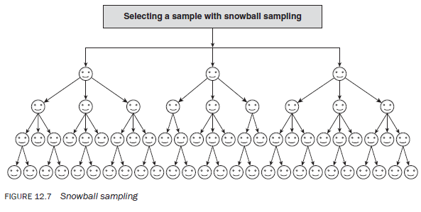
Snowball sampling is the process of selecting a sample using networks. To start with, a few indi­viduals in a group or organisation are selected and the required information is collected from them. They are then asked to identify other people in the group or organisation, and the people selected by them become a part of the sample. Information is collected from them, and then these people are asked to identify other members of the group and, in turn, those identified become the basis of further data collection (Figure 12.7). This process is continued until the required number or a saturation point has been reached, in terms of the information being sought.

This sampling technique is useful if you know little about the group or organisation you wish to study, as you need only to make contact with a few individuals, who can then direct you to the other members of the group. This method of selecting a sample is useful for studying communication patterns, decision making or diffusion of knowledge within a group. There are disadvantages to this technique, however. The choice of the entire sample rests upon the choice of individuals at the first stage. If they belong to a particular faction or have strong biases, the study may be biased. Also, it is difficult to use this technique when the sample becomes fairly large.

8. Systematic sampling design: a ‘mixed’ design

Systematic sampling has been classified as a ‘mixed’ sampling design because it has the characteristics of both random and non-random sampling designs.

In systematic sampling the sampling frame is first divided into a number of segments called intervals. Then, from the first interval, using the SRS technique, one element is selected. The selection of subsequent elements from other intervals is dependent upon the order of the ele­ment selected in the first interval. If in the first interval it is the fifth element, the fifth element
of each subsequent interval will be chosen. Notice that from the first interval the choice of an element is on a random basis, but the choice of the elements from subsequent intervals is dependent upon the choice from the first, and hence cannot be classified as a random sample. The procedure used in systematic sampling is presented in Figure 12.8.

Although the general procedure for selecting a sample by the systematic sampling tech­nique is described above, you can deviate from it by selecting a different element from each interval with the SRS technique. By adopting this, systematic sampling can be classified under probability sampling designs.

To select a random sample you must have a sampling frame (Figure 12.9). Sometimes this is impossible, or obtaining one may be too expensive. However, in real life there are situations where a kind of sampling frame exists, for example records of clients in an agency, enrolment lists of students in a school or university, electoral lists of people living in an area, or records of the staff employed in an organisation. All these can be used as a sampling frame to select a sample with the systematic sampling technique. This convenience of having a ‘ready-made’ sampling frame may be at a price: in some cases it may not truly be a random listing. Mostly these lists are in alphabetical order, based upon a number assigned to a case, or arranged in a way that is convenient to the users of the records. If the ‘width of an interval’ is large, say, 1 in 30 cases, and if the cases are arranged in alphabetical order, you could preclude some whose surnames start with the same letter or some adjoining letter may not be included at all.

Suppose there are 50 students in a class and you want to select 10 students using the system­atic sampling technique. The first step is to determine the width of the interval (50/10 = 5). This means that from every five you need to select one element. Using the SRS technique, from the first interval (1—5 elements), select one of the elements. Suppose you selected the third element. From the rest of the intervals you would select every third element.

9. The calculation of sample size

Students and others often ask: ‘How big a sample should I select?’, ‘What should be my sample size?’ and ‘How many cases do I need?’ Basically, it depends on what you want to do with the findings and what type of relationships you want to establish. Your purpose in undertaking research is the main determinant of the level of accuracy required in the results, and this level of accuracy is an important determinant of sample size. However, in qualitative research, as the main focus is to explore or describe a situation, issue, process or phenomenon, the question of sample size is less important. You usually collect data till you think you have reached saturation point in terms of discovering new information. Once you think you are not getting much new data from your respondents, you stop collecting further information. Of course, the diversity or heterogeneity in what you are trying to find out about plays an important role in how fast you will reach saturation point. And remem­ber: the greater the heterogeneity or diversity in what you are trying to find out about, the greater the number of respondents you need to contact to reach saturation point. In determining the size of your sample for quantitative studies and in particular for cause-and-effect studies, you need to consider the following:

• At what level of confidence do you want to test your results, findings or hypotheses?
• With what degree of accuracy do you wish to estimate the population parameters?
• What is the estimated level of variation (standard deviation), with respect to the main variable you are studying, in the study population?

Answering these questions is necessary regardless of whether you intend to determine the sample size yourself or have an expert do it for you. The size of the sample is important for testing a hypothesis or establishing an association, but for other studies the general rule is: the

larger the sample size, the more accurate your estimates. In practice, your budget determines the size of your sample. Your skills in selecting a sample, within the constraints of your budget, lie in the way you select your elements so that they effectively and adequately represent your sampling population.

To illustrate this procedure let us take the example of a class. Suppose you want to find out the average age of the students within an accuracy of 0.5 of a year; that is, you can tolerate an error of half a year on either side of the true average age. Let us also assume that you want to find the average age within half a year of accuracy at the 95 per cent confidence level; that is, you want to be 95 per cent confident about your findings.

The formula (from statistics) for determining the confidence limits is

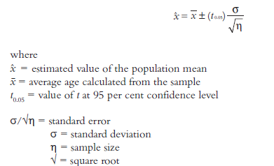
If we decide to tolerate an error of half a year, that means

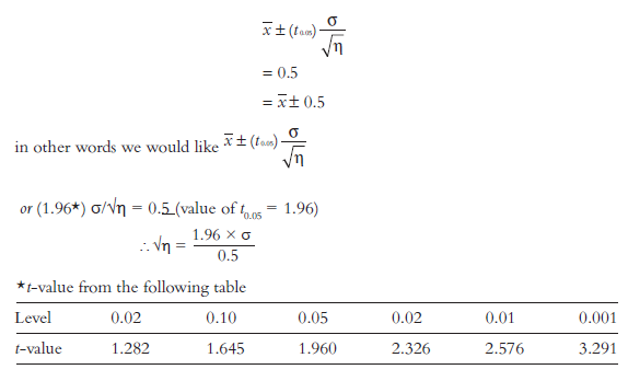
Now the main problem is to find the value of ct without having to collect data. This is the biggest problem in estimating the sample size. Because of this it is important to know as much as possible about the study population.

The value of ct can be found by one of the following:

1. guessing;
2. consulting an expert;
3. obtaining the value of ct from previous comparable studies; or
4. carrying out a pilot study to calculate the value.

Let us assume that ct is 1 year. Then

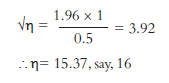
Hence, to determine the average age of the class at a level of 95 per cent accuracy (assuming ct = 1 year) with half a year of error, a sample of at least 16 students is necessary.

Now assume that, instead of 95 per cent, you want to be 99 per cent confident about the estimated age, tolerating an error of half a year. Then

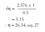
Hence, if you want to be 99 per cent confident and are willing to tolerate an error of half a year, you need to select a sample of 27 students. Similarly, you can calculate the sample size with varying values of ct. Remember the golden rule: the greater is the sample size, the more accurately your findings will reflect the ‘true’ picture.

Source: Kumar Ranjit (2012), Research methodology: a step-by-step guide for beginners, SAGE Publications Ltd; Third edition.