Sharing Risk and Reward in the Supply Chain

In this chapter so far, we have emphasized the fact that all sourcing decisions should be made with the goal of growing the supply chain surplus. In practice, however, many firms care less about growing the surplus and more about what share of the surplus they are able to capture. As firms gain greater power in a supply chain, they often attempt to capture a greater share of the surplus while pushing more risk onto their supply chain partners. In this section, we focus on the downsides of focusing on a firm’s local interest at the expense of the supply chain sur­plus. We also suggest some approaches that can be used to counter the downsides of local optimization.

1. Sharing Risk to grow Supply chain profits

Independent actions taken by two parties in a supply chain often result in profits that are lower than those that could be achieved if the supply chain were to coordinate its actions with a common objective of maximizing supply chain profits rather than individual firm profits. As firms get stronger, they tend to push more risk on to supply chain partners while keeping a large margin for themselves. A classic example of such an approach is the action taken by Mattel in 1999 in response to adverse outcomes in 1998. Until 1998, Mattel allowed its retailers to place two orders for the Christmas season. Mattel delivered the first order before the Thanksgiving weekend; retailers then placed their second order after observing sales over that weekend. The weekend sales allowed retailers to get a much better forecast for the Christmas season before placing the second order. In 1998, sales over the Thanksgiv­ing weekend were soft and many retailers decided not to place a second order. As a result, Mattel reported a $500 million sales shortfall in the last weeks of the year. Having been burned because of its willingness to absorb the risk of the second order, Mattel changed its policy for 1999. It now required retailers to place their entire order before Thanksgiving and the company would take no reorders in December. Mattel announced that the new policy would allow the company to “tailor production more closely to demand and avoid building inventory for orders that don’t come.”

The actions of Mattel amounted to shifting risk from Mattel to the retailers. Whereas Mattel absorbed some of the forecast uncertainty when retailers were allowed a follow-up order in December, forcing retailers to place their orders before Thanksgiving pushed all the risk of fore­cast error onto them. This action by Mattel (seemingly taken because of its self-interest) clearly hurts retailers. We now argue that it also hurts Mattel. Given demand uncertainty, a manufacturer like Mattel wants the retailer to carry a large inventory of its product to ensure that any surge in demand can be satisfied. The retailer, on the other hand, loses money on any unsold inventory. As a result, the retailer prefers to carry a lower level of inventory, especially when it must absorb the entire risk of a forecast error. This tension leads to a supply chain outcome that hurts both the retailer and the manufacturer, as illustrated in Example 15-1 (see worksheet Example15-1 in workbook Chapter15-examples).

EXAMPLE 15-1 Impact of Local Optimization

Consider a music store that sells compact discs. The supplier manufactures compact discs at $1 per unit and sells them to the music store at $5 per unit. The retailer sells each disc to the end consumer at $10. At this retail price, market demand is normally distributed, with a mean of 1000 and a standard deviation of 300. Any leftover discs at the end of the sale period are worth­less. How many discs should an independent retailer order? What are the supply chain profits with an independent retailer? If the manufacturer and the retailer are vertically integrated (they are a single firm), how many discs should the retailer order? What are the supply chain profits when the manufacturer and retailer are a single firm?

Analysis:

We first consider the case of the independent retailer. The retailer has a margin of $5 per disc and can potentially lose $5 for each unsold disc. The retailer thus has a cost of overstocking C_o = $5 and a cost of understocking C_u = $5. Using Equation 13.1, it is optimal for the retailer to aim for a service level of 5 / (5 + 5) = 0.5 and order NORMINV(0.5, 1000, 300) = 1,000 discs. From Equation 13.3, the retailer’s expected profits are $3,803, and the manufacturer makes $4,000 from selling 1,000 discs. The total supply chain profit with an independent retailer is thus $3,803 + $4,000 = $7,803.

Now, consider the case in which the supply chain is vertically integrated. The supply chain has a margin of $10 – $1 = $9 per disc and can potentially lose $1 for each unsold disc. The supply chain thus has a cost of overstocking C_o = $1 and a cost of understocking C_u = $9. Using Equation 13.1, it is optimal for the supply chain to aim for a service level of 9 / (1 + 9) = 0.9 and order NORMINV(0.9, 1000, 300) = 1,384 discs. From Equation 13.3, the supply chain’s expected profits are $8,474.

Thus, the vertically integrated supply chain makes $670 more than when the retailer makes the ordering decision independently.

As discussed in Chapter 11, double marginalization reduces supply chain profits because the supply chain margin is divided between the two parties, and each stage makes its decisions considering only its own margin. We now discuss several other instances in which double mar­ginalization leads to a loss in supply chain performance in the presence of demand uncertainty.

An independent retailer makes its buying decision before demand is realized and thus bears all the demand uncertainty. If demand is less than the retailer’s inventory, the retailer must liquidate unsold product at a discount. Given uncertain demand, the retailer decides on the pur­chase quantity based on its margin and the cost of overstocking, as discussed in Chapter 13. The retailer’s margin, however, is lower than the contribution margin for the entire supply chain, whereas its cost of overstocking is higher than that for the entire supply chain. As a result, the retailer is conservative and aims for a lower level of product availability than is optimal for the supply chain leading to a loss of supply chain surplus. As Example 15-1 illustrates, if the retailer absorbs all the risk of forecast error while getting only a portion of the margin ($4 in this exam­ple, compared with a supply chain margin of $9), the retailer’s ordering decision lowers supply chain profits compared with those of a vertically integrated supply chain.

From our discussion, it seems clear that Mattel’s actions—in which it pushed all the risk onto retailers—clearly hurt supply chain profits because retailers were more conservative than they would have been when Mattel shared some risk. The conservative approach of the retailers did not allow the supply chain to take advantage of any upside in demand, thus reducing supply chain profits.

Given that we have identified the problem when risk is not shared, we now focus on iden­tifying potential solutions that allow for risk sharing in a way that increases supply chain profits. To improve overall profits, the supplier must share risk in a way that encourages the buyer to purchase more and increase the level of product availability. This requires the supplier to share in some of the buyer’s demand uncertainty. The following three approaches to risk sharing increase overall supply chain profits:

1. Buybacks or returns
2. Revenue sharing
3. Quantity flexibility

We illustrate each of the three approaches using the story in Example 15-1 of the music store. We discuss the performance of each approach in terms of the following three questions.

1. How will risk sharing affect the firm’s profits and total supply chain profits?
2. Will risk sharing introduce any information distortion?
3. How will risk sharing influence supplier performance along key performance measures?

RISK SHARING THROUGH BUYBACKS A buyback or returns clause allows a retailer to return unsold inventory up to a specified amount, at an agreed-upon price. In this case, the supplier is sharing risk by agreeing to buy back unsold inventory at the retailer. In a buyback contract, the manufacturer specifies a wholesale price c along with a buyback price b at which the retailer can return any unsold units at the end of the season. We assume that the manufacturer can salvage $s_M for any units that the retailer returns. The manufacturer has a cost of v per unit produced. The retail price is p.

The optimal order quantity O* for a retailer in response to a buyback contract is evaluated using Equations 13.1 and 13.2, where the salvage value for the retailer is s = b. The cost of overstocking for the retailer is given by C_o = c — b, and the cost of understocking for the retailer is given by C_u = p — c. Using Equation 13.1, the optimal service level that the retailer targets is thus given by CSL* = (p — c) / (p — b). Using Equation 13.2, the optimal order size by the retailer is given by O* = NORMINV(CSL*, m, s). The expected retailer profit is evalu­ated using Equation 13.3 with the salvage value s equal to the buyback price b. The expected profit at the manufacturer depends on the overstock at the retailer (evaluated using Equation 13.4) that is returned. We obtain

We illustrate the impact of buybacks on supply chain profits in Example 15-2 (see work­sheet Example15-2).

EXAMPLE 15-2 Impact of Risk Sharing Through Buybacks

We return to the music store in Example 15-1 with all data as specified. Assume that the supplier agrees to buy back any unsold discs for $3 even though any leftover discs at the end of the sale period are worthless. With the buyback clause, how many discs should an independent retailer order? What are the supply chain profits with a buyback clause?

Analysis:

With a buyback clause as specified, the retailer has a salvage value of $3 for each unsold unit. Given the wholesale price of $5 and a retail price of $10, the retailer thus has a cost of overstock­ing, C_o = $5 – $3 = $2 and a cost of understocking C_u = $10 — $5 = $5. Using Equation 13.1, it is optimal for the retailer to aim for a service level of 5 / (2 + 5) = 0.71 and order 1,170 [ = NORMlNV(5/7, 1000, 300)] discs. From Equation 13.3, the retailer’s expected profits are $4,286. Given an expected overstock of 223 units (using Equation 13.4), the manufacturer’s expected profit is $4,011 [ = 1170 X (5 – 1) – (223 X 3)]. The total supply chain profit with buybacks is thus $4,286 + $4,011 = $8,297.

Observe that risk sharing using a buyback clause for $3 increases profits for the retailer as well as the manufacturer (and the supply chain as a whole) compared with Example 15-1, in which there was no risk sharing.

Example 15-2 illustrates that risk sharing through a suitably designed buyback clause can increase manufacturer profits (relative to the case without risk sharing) even though the retailer is compensated for any unsold inventory. Risk sharing by the manufacturer always increases the retailer’s profits increase because the retailer’s cost of overstocking has decreased. Despite buy­ing back unsold inventory at $3, the supplier’s profits increase in Example 15-2 because the retailer, on average, sells more product (on which the supplier makes $5 per unit). Buyback con­tracts are most effective for products with a low variable cost, such as music, software, books, magazines, and newspapers.

Table 15-3 (which can be constructed using worksheet Example15-2) shows supply chain profits for different values of wholesale and buyback prices. Observe that the use of buyback contracts increases total supply chain profits by about 20 percent when the wholesale price is $7 per disc. For a fixed wholesale price, increasing the buyback price always increases retailer prof­its. In general, there exists a positive buyback price that is a fraction of the wholesale price, at which the manufacturer makes a higher profit compared to offering no buyback. Also observe that buybacks increase profits for the manufacturer more as the manufacturer’s margin increases. In Table 15-3, buybacks are found to be more helpful to the manufacturer when the who lesaleprice is $7 relative to when the wholesale price is $5. Thus, the greater the manufacturer’s mar­gin, the more the manufacturer stands to benefit through the use of some risk-sharing mechanism such as buybacks.

For a fixed wholesale price, as the buyback price increases, the retailer orders more and also returns more. In our analysis in Table 15-3, though, we have not considered the cost associ­ated with a return. As the cost associated with a return increases, buyback contracts become less attractive because the cost of returns reduces supply chain profits. If return costs are high, buy­back contracts can reduce the total profits of the supply chain far more than is the case without any buyback.

In 1932, Viking Press was the first book publisher to accept returns. Today, buyback con­tracts are common in the book industry, and publishers accept unsold books from retailers. To minimize the cost associated with a return, retailers do not have to return the book, only the cover. When publishers can verify retailer sales electronically, nothing must be returned. The goal in either case is for the publisher to get proof that the book did not sell while reducing the cost of the return. Over the years, considerable debate has taken place about the impact of pub­lishers’ returns policy on profits in the industry. Our discussion provides some justification for the approach taken by the publishers.

In some instances, manufacturers use holding-cost subsidies or price protection to share risk and encourage retailers to order more. With holding-cost subsidies, manufacturers pay retailers a certain amount for every unit held in inventory over a given period. Holding-cost subsidies are prevalent in automotive supply chains. In the high-tech industry, in which prod­ucts lose value rapidly, manufacturers share the risk of product becoming obsolete by providing price support to retailers. Many manufacturers guarantee that in the event that they drop prices, they will also lower prices for all inventories that the retailer is currently carrying and compen­sate the retailer accordingly. As a result, the cost of overstocking at the retailer is limited to the cost of capital and physical storage and does not include obsolescence, which can be more than 100 percent a year for high-tech products. The retailer thus increases the level of product avail­ability in the presence of price support. Both holding-cost subsidies and price support are forms of buyback.

A downside to the buyback clause (or any equivalent practice, such as holding-cost sub­sidy or price support) is that it leads to surplus inventory that must be salvaged or disposed. The task of returning unsold product increases supply chain costs. The cost of returns can be elimi­nated if the manufacturer gives the retailer a markdown allowance and allows it to sell the prod­uct at a significant discount. Publishers today generally do not ask retailers to return unsold books; instead, they give a markdown allowance for them. Retailers then mark them down and sell them for a considerable discount.

For a given level of product availability at the retailer, the presence of a buyback clause can also hurt sales because it leads the retailer to exert less effort to sell than it would without buy­backs. The reduction in retailer effort in the presence of buyback occurs because its loss from unsold inventory is higher when there is no buyback, leading to a higher sales effort for products with no buyback. The supplier can counter the reduction in sales effort by limiting the amount of buyback permitted.

The structure of a buyback clause leads to the entire supply chain reacting to the order placed by the retailer and not to actual customer demand. If a supplier is selling to multiple retailers, it produces based on the orders placed by each retailer. Each retailer bases its order on its cost of overstocking and understocking (see Chapter 13). After actual sales materialize, unsold inventory is returned to the supplier separately from each retailer. As a result, the structure of the buyback clause increases information distortion when a supplier is selling to multiple retailers. At the end of the sales season, however, the supplier does obtain information on actual sales. Information distortion is driven primarily by the fact that inventory is disaggregated at the retail­ers based on an ordering decision made when demand is uncertain. If inventory is produced by the supplier and sent out only as needed to the retailers, information distortion can be reduced.

With more responsive production and centralized inventory, the supplier can exploit indepen­dence of demand across retailers to carry a lower level of inventory. In practice, however, most buyback contracts have decentralized inventory at retailers. As a result, there is a high level of information distortion.

RISK SHARING THROUGH REVENUE SHARING In revenue-sharing contracts, the manufac­turer charges the retailer a lower wholesale price c (compared with the case without risk sharing), but shares a fraction f of the retailer’s revenue. In this case, the manufacturer is sharing risk because the retailer’s cost is lower (than without risk sharing) if demand is low. Even if no returns are allowed, the lower wholesale price decreases the cost to the retailer in case of an over­stock. The retailer thus increases the level of product availability, resulting in higher profits for both the manufacturer and the retailer when revenue sharing is suitably designed.

Assume that the manufacturer has a production cost v; the retailer charges a retail price p and can salvage any leftover units for s_R. The optimal order quantity O* ordered by the retailer is evaluated using Equations 13.1 and 13.2, where the cost of understocking is C_u = (1 – f)p — c and the cost of overstocking is C_o = c — s_R. We thus obtain

The manufacturer obtains the wholesale price c for each unit purchased by the retailer and a share of the revenue for each unit sold by the retailer. The expected overstock at the retailer is obtained using Equation 13.4. The manufacturer’s profits are thus evaluated as

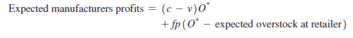
The retailer pays a wholesale price c for each unit purchased and obtains a revenue of 11 – f2p for each unit sold and a revenue of sR for each unit overstocked. The retailer’s expected profit is thus evaluated as

We illustrate the impact of revenue sharing on supply chain profits using Example 15-3 (see worksheet Example15-3).

EXAMPLE 15-3 Impact of Risk Sharing Through Revenue Sharing

We return to the music store in Example 15-1 with all data as specified. Assume that the supplier agrees to a revenue sharing contract under which the retailer is charged only $1 for each disc, with the manufacturer getting 45 percent of the retail revenues. Given the retail price of $10, the manufacturer gets $4.50 for each disc sold while the retailer keeps $5.50. With the revenuesharing clause, how many discs should an independent retailer order? What are the supply chain profits with a revenue-sharing clause?

Analysis:

With a revenue-sharing clause as specified, we have c = $1, p = $10, sR = 0, and a revenue share fraction f = 0.45. The manufacturer has a production cost of v = $1. The music store thus has a cost of overstocking of Co = c – sR = 1 – 0 = $1 and a cost of understocking of Cu = (1 – f)p – c = (1 – 0.45) * 10 – 1 = $4.50. The music store targets a service level of CSL* = 4.5 / (4.5 + 1) = 0.818, or 81.8 percent (see Equation 13.1) and orders 1,273 [ = NORMINV(4.5 /5.5, 1000, 300)] discs. Observe that this is much larger than the 1,000 discs ordered in Example 15-1, when the wholesale price was $5 and there was no revenue sharing. The increase in order size occurs because the retailer loses only $1 per unsold disc (instead of $5 per disc without revenue sharing), while making a margin of $4.50 for each disc that sells.

Given an order of 1,273 discs, the retailer has an expected overstock of 302 discs (use Equation 13.4). As a result, the expected manufacturer’s profit = (c — v)O* + fp(O*- expected overstock = (1 — 1) X 1273 + 0.45 X 10 X (1273 — 302) = $4,369. The expected retailer’s profit = (1 — f) p(O* — expected overstock at retailer) + s_R X expected overstock at retailer — cO* = (1 — 0.45) X 10 X (1273 — 302) + 0 X 302 — 1 X 1273 = $4,068. The total supply chain profit = 4,369 + 4,068 = $8,437.

Observe that risk sharing using a revenue sharing clause with a $1 wholesale price and a 45 percent share for the supplier increases profits for the retailer as well as the manufacturer (and the supply chain as a whole) compared with Example 15-1, in which there was no risk sharing.

Table 15-4 (constructed using worksheet Example15-3 in spreadsheet Chapter15- examples) provides the outcome in terms of order sizes and profits for different wholesale prices and revenue-sharing fractions f. From Tables 15-3 and 15-4, observe that revenue sharing allows both the manufacturer and retailer to increase their profits in the absence of buybacks compared with the case in which the wholesaler sells for a fixed price of $5 without buybacks. Recall that when charging a wholesale price of $5, the supplier makes profit of $4,000 and the music store makes a profit of $3,803 (see Table 15-3).

Revenue-sharing contracts also result in lower retailer effort compared with the case in which the retailer pays an upfront wholesale price and keeps the entire revenue from a sale. The drop in effort results because the retailer gets only a fraction of the revenue from each sale. One advantage of revenue-sharing contracts over buyback contracts is that no product needs to be returned, thus eliminating the cost of returns. Revenue-sharing contracts are best suited for prod­ucts with low variable cost and a high cost of return. A good example of revenue-sharing con­tracts was implemented between Blockbuster video rentals and movie studios for videos. A studio sold each cassette to Blockbuster at a low price and then shared in the revenue generated from each rental. Given the low price, Blockbuster purchased many copies, resulting in more rentals and higher profits for both Blockbuster and the studio.

The revenue-sharing contract does require an information infrastructure that allows the sup­plier to monitor sales at the retailer. Such an infrastructure can be expensive to build. As a result, revenue-sharing contracts may be difficult to manage for a supplier selling to many small buyers.

As in buyback contracts, revenue-sharing contracts also result in the supply chain produc­ing to retailer orders rather than to actual consumer demand. This information distortion results in excess inventory in the supply chain and a greater mismatch between supply and demand. The information distortion increases as the number of retailers to which the supplier sells grows. As with buyback contracts, information distortion from revenue-sharing contracts can be reduced if retailers reserve production capacity or inventory at the supplier rather than buying product and holding it in inventory themselves. This allows aggregation of the variability across multiple retailers, and the supplier must hold a lower level of capacity or inventory. In practice, however, most revenue-sharing contracts are implemented with the retailer buying and holding inventory.

RISK SHARING USING QUANTITY FLEXIBILITY Under quantity flexibility contracts, the manufac­turer allows the retailer to change the quantity ordered (within limits) after observing demand. If a retailer orders O units, the manufacturer commits to providing up to Q = (1 + a)O units, whereas the retailer is committed to buying at least q = (1 – b)O units. Both a and b are between 0 and 1. The retailer can purchase anywhere between q and Q units, depending on the demand it observes. Quantity flexibility contracts are similar in spirit to the contract that Mattel offered its retailers prior to 1999. In quantity flexibility contracts the manufacturer shares risk by allowing the retailer to adjust its order as better market information is received. Because no returns are required, these con­tracts can be more effective than buyback contracts when the cost of returns is high. When the sup­plier is selling to multiple retailers, these contracts are more effective than buyback contracts because they allow the supplier to aggregate uncertainties across multiple retailers and thus lower the level of excess inventory. Quantity flexibility contracts increase the average amount the retailer purchases and may increase total supply chain profits when structured appropriately.

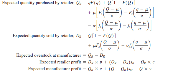
Assume that the manufacturer incurs a production cost of $v per unit and charges a whole­sale price of $c from the retailer. The retailer, in turn, sells to customers for a price of $p. The retailer salvages any leftover units for s_R. The manufacturer salvages any leftover units for s_M. If retailer demand is normally distributed, with a mean of m and a standard deviation of s, we can evaluate the impact of a quantity flexibility contract. If the retailer orders O units, the manufac­turer is committed to supplying Q units. As a result, we assume that the manufacturer produces Q units. The retailer purchases q units if demand D is less than q, D units if demand D is between q and Q, and Q units if demand D is greater than Q. In the following formulas, F_S is the standard normal cumulative distribution function and fS is the standard normal density function discussed in Appendix 12A in Chapter 12. We thus obtain

We illustrate the impact of quantity flexibility on supply chain profits using Example 15-4 (see worksheet Example15-4).

EXAMPLE 15-4 Impact of Risk Sharing Through Quantity Flexibility

We return to the music store in Example 15-1 with all data as specified. The retailer is charged $5 for each disc and has a retail price of $10. Assume that the supplier agrees to a quantity flexibility

contract where the supplier agrees to a = 0.05 and b = 0.05. For this contract, the retailer decides to place an order for 1,017 units. With the quantity flexibility clause, how many discs does the independent retailer expect to purchase? How many discs does the retailer expect to sell? What are the supply chain profits with a quantity flexibility clause?

Analysis:

In this case, we have v = $1, c = $5, p = $10, s_R = 0, and s_M = 0. With the quantity flexibil­ity clause as specified, and an order for O = 1,017 from the retailer, the manufacturer is com­mitted to supplying any quantity between q = (1 – b)O = (1 – 0.05) X 1017 = 966 units and Q = (1 + a)O = (1 + 0.05) X 1017 = 1,068 units. We thus obtain

Expected quantity purchased by retailer, Q_R = 1,015 units

Expected quantity sold by retailer, D_R = 911 units

Expected overstock at retailer = Q_R — D_R = 1,015 – 911 = 104 units

Given an order of 1,017 discs (which is adjusted between 966 and 1,068 based on actual demand), the total supply chain profit = 4,038 + 4,007 = $8,045.

Observe that risk sharing using a quantity flexibility clause with a flexibility of 5 percent above and below the order quantity increases profits for the retailer as well as the manufacturer (and the supply chain as a whole) compared with Example 15-1, in which there was no risk sharing.

With a quantity flexibility clause, the retailer is able to take advantage of market intelli­gence so the amount finally purchased by the retailer is more in line with actual demand. The better matching of supply and demand results in higher profits for the retailer. If the supplier has access to some flexible and responsive capacity, it can produce the uncertain part of the order after the retailer order is finalized while producing the base load (q units) using an inexpensive production method. This tailoring of production allows the supplier to reduce overall costs. A quantity flexibility contract is particularly effective if a supplier is selling to multiple retailers with independent demand because it allows uncertainties to be aggregated by the supplier.

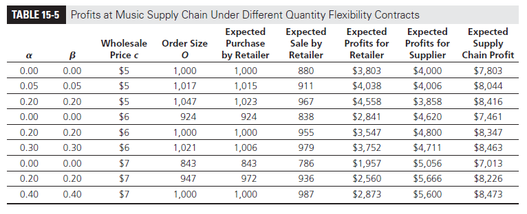
In Table 15-5, we show the impact of different quantity flexibility contracts on profit­ability for the music supply chain when demand is normally distributed, with a mean of m = 1,000 and a standard deviation of s = 300 (see worksheet Example15-4 in spreadsheet Chapter15-examples). We assume a wholesale price of c = $5 and a retail price of p = $10. All contracts considered are such that a = fi. The results in Table 15-5 are built in two steps. We first fix a and b (say a = b = 0.2). The next step is to identify the optimal order size for the retailer. This is done using Excel by selecting an order size that maximizes expected retailer profits given a and b. For example, when a = b = 0.05 and c = $5, retailer profits are max­imized for an order size of O = 1,017. For this order size, we obtain a supplier commitment to deliver up to Q = (1 + 0.05) X 1,017 = 1,068 and a retailer commitment to buy at least q = (1 – 0.05) X 1,017 = 966 discs. In our analysis, we assume that the supplier produces Q = 1,068 discs and sends the precise number (between 966 and 1,068) demanded by the retailer. Such a policy results in retailer profits of $4,038 and supplier profits of $4,006.

From Table 15-5, observe that quantity flexibility contracts allow both the manufacturer and the retailer to increase their profits. Observe that as the manufacturer increases the wholesale price, it is optimal for it to offer greater quantity flexibility to the retailer.

Quantity flexibility contracts are common for components in the electronics and computer industries. In the previous discussion, we considered fairly simple quantity flexibility contracts. Benetton has used sophisticated quantity flexibility contracts with its retailers successfully to increase supply chain profits. We describe such a contract in the context of colored knit garments (see Heskett and Signorelli, 1984).

Seven months before delivery, Benetton retailers were required to place their orders. Con­sider a retailer placing an order for 100 sweaters each in red, blue, and yellow. One to three months before delivery, retailers could alter up to 30 percent of the quantity ordered in any color and assign it to another color. The aggregate order, however, could not be adjusted at this stage. Potentially, the retailer could change the order to 70 red, 70 blue, and 160 yellow sweaters. After the start of the sales season, retailers were allowed to order up to 10 percent of their previous order in any color. Potentially, then, the retailer could order another 30 yellow sweaters. In this quantity flexibility contract, Benetton retailers had a flexibility of up to 10 percent on the aggre­gate order across all colors and of about 40 percent for individual colors. Retailers could increase the aggregate quantity ordered by up to 10 percent, and the quantity for any individual color could be adjusted by up to 40 percent. This flexibility is consistent with the fact that aggregate forecasts are more accurate than forecasts for individual colors. As a result, retailers could better match product availability with demand. The guaranteed portion of the order was manufactured by Benetton using an inexpensive but long-lead-time production process. The flexible part of the order (about 35 percent) was manufactured using postponement. The result was a better match­ing of supply and demand at lower cost than in the absence of quantity flexibility. The quantity flexibility contract allowed both the retailers and Benetton to increase their profits.

The quantity flexibility contract requires either inventory or excess flexible capacity to be available at the supplier. If the supplier is selling to multiple retailers with independent demand, the aggregation of inventory leads to a smaller surplus inventory (see Chapter 12) with a quantity flexibility contract compared to either a buyback or revenue-sharing contract. Inventories can be further reduced if the supplier has excess flexible capacity. Quantity flexibility contracts are thus preferred for products with high marginal cost or when surplus capacity is available. To be effec­tive, quantity flexibility contracts require the retailer to be good at gathering market intelligence and improving its forecasts closer to the point of sale.

Relative to buyback and revenue-sharing contracts, quantity flexibility contracts have less information distortion. Consider the case with multiple retailers. With a buyback contract, the supply chain must produce based on the retailer orders that are placed well before actual demand arises. This leads to surplus inventory being disaggregated at each retailer. With a quantity flex­ibility contract, retailers specify only the range within which they will purchase, well before actual demand arises. If demand at various retailers is independent, the supplier does not need to plan production to the high end of the order range for each retailer. It can aggregate uncertainty across all retailers and build a lower level of surplus inventory than would be needed if inventory were disaggregated at each retailer. Retailers then order closer to the point of sale, when demand is more visible and less uncertain. The aggregation of uncertainty results in less information dis­tortion with a quantity flexibility contract.

As with the other contracts discussed, quantity flexibility contracts result in lower retailer effort. In fact, any contract that gets retailers to provide a higher level of product availability by not making them fully responsible for overstocking will result in a lowering of retailer effort for a given level of inventory.

Key Point

Risk sharing in a supply chain increases profits for both the supplier and the retailer. Risk sharing mechanisms include buybacks, revenue sharing, and quantity flexibility. Quantity flexibility contracts result in lower information distortion than buyback or revenue-sharing contracts when a supplier sells to multiple buyers or the supplier has excess, flexible capacity.

2. Sharing Rewards to improve Performance

Having discussed the benefits of sharing risk, we now focus on the importance of sharing rewards in a supply chain. In many instances, a buyer wants performance improvement from a supplier that has little incentive to do so. A supplier may be reluctant to invest in improvement if the effort for improvement must be exerted by the supplier but most of the benefits from improvement accrue to the buyer. In such a setting, sharing the benefits from improvement can encourage sup­plier cooperation, resulting in a better supply chain outcome.

As an example, consider a buyer that wants the supplier to improve performance by reduc­ing lead time for a seasonal item. This is an important component of all quick response initiatives in a supply chain. With a shorter lead time, the buyer hopes to have better forecasts and be better able to match supply and demand. Most of the work to reduce lead time must be done by the sup­plier, whereas most of the benefit accrues to the buyer in terms of reduced inventories, overstock­ing, and lost sales. In fact, the supplier will lose sales because the buyer will now carry less safety inventory as a result of shorter lead times and better forecasts. To induce the supplier to reduce lead time, the buyer can use a shared-savings contract, with the supplier getting a fraction of the savings that result from reducing lead time. As long as the supplier’s share of the savings compensates for any effort it has to put in, its incentive will be aligned with that of the buyer, resulting in an outcome that benefits both parties.

A similar issue arises when a buyer wants to encourage the supplier to improve quality. Improving supply quality reduces the buyer’s costs but requires additional effort from the sup­plier. Once again, a shared-savings contract is a good way to align incentives between the buyer and supplier. The buyer can share savings from improved quality with the supplier. This will encourage the supplier to improve quality to a higher level than what the supplier would choose in the absence of the shared savings.

Another example arises in the context of toxic chemicals that may be used by a manufac­turer. The manufacturer would like to decrease the use of these toxic chemicals. Generally, the supplier is better equipped to identify ways of reducing use of these chemicals, because this is its core business. It has no incentive to work with the buyer on reducing use of these chemicals, however, because that will reduce the supplier’s sales. A shared-savings contract can be used to align incentives between the supplier and the manufacturer. If the manufacturer shares the sav­ings that result from a reduction in the use of toxic chemicals with the supplier, the supplier will make the effort to reduce use of the chemicals as long as its share of the savings compensates for the loss in margin from reduced sales.

In general, sharing the savings is effective in aligning supplier and buyer incentives when the supplier is required to improve performance along a particular dimension and most of the benefits of improvement accrue to the buyer. A powerful buyer may couple shared savings with penalties for a lack of improvement to further encourage the supplier to improve performance. Sharing the rewards of improvements increases profits for both the buyer and the supplier while achieving outcomes that are beneficial to the supply chain.

Key Point

Sharing the rewards from improvements can induce performance improvement from a supplier along dimensions, such as lead time, for which the benefit of improvement accrues primarily to the buyer but the effort for improvement comes primarily from the supplier.

Source: Chopra Sunil, Meindl Peter (2014), Supply Chain Management: Strategy, Planning, and Operation, Pearson; 6th edition.