Decision Analysis with Sample Information

In applying the expected value approach, we showed how probability information about the states of nature affects the expected value calculations and thus the decision recommenda­tion. Frequently, decision makers have preliminary or prior probability assessments for the states of nature that are the best probability values available at that time. However, to make the best possible decision, the decision maker may want to seek additional informa­tion about the states of nature. This new information can be used to revise or update the prior probabilities so that the final decision is based on more accurate probabilities for the states of nature. Most often, additional information is obtained through experiments de­signed to provide sample information about the states of nature. Raw material sampling, product testing, and market research studies are examples of experiments (or studies) that may enable management to revise or update the state-of-nature probabilities. These revised probabilities are called posterior probabilities.

Let us return to the PDC problem and assume that management is considering a six-month market research study designed to learn more about potential market acceptance of the PDC condominium project. Management anticipates that the market research study will provide one of the following two results:

1. Favorable report: A significant number of the individuals contacted express interest in purchasing a PDC condominium.
2. Unfavorable report: Very few of the individuals contacted express interest in pur­chasing a PDC condominium.

1. Decision Tree

The decision tree for the PDC problem with sample information shows the logical sequence for the decisions and the chance events in Figure 19.4. First, PDC’s management must decide whether the market research should be conducted. If it is conducted, PDC’s management must be prepared to make a decision about the size of the condominium project if the market re­search report is favorable and, possibly, a different decision about the size of the condominium project if the market research report is unfavorable.

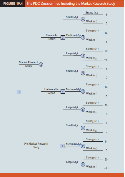
In Figure 19.4, the squares are decision nodes and the circles are chance nodes. At each decision node, the branch of the tree that is taken is based on the decision made. At each chance node, the branch of the tree that is taken is based on probability or chance. For example, decision node 1 shows that PDC must first make the decision whether to conduct the market research study. If the market research study is under­taken, chance node 2 indicates that both the favorable report branch and the unfavor­able report branch are not under PDC’s control and will be determined by chance.

Node 3 is a decision node, indicating that PDC must make the decision to construct the small, medium, or large complex if the market research report is favorable. Node 4 is a decision node showing that PDC must make the decision to construct the small, medium, or large complex if the market research report is unfavorable. Node 5 is a decision node indicating that PDC must make the decision to construct the small, medium, or large complex if the market research is not undertaken. Nodes 6 to 14 are chance nodes indicating that the strong demand or weak demand state-of-nature branches will be determined by chance.

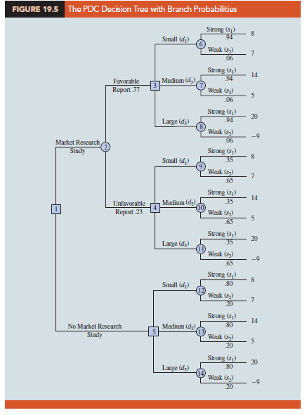
Analysis of the decision tree and the choice of an optimal strategy requires that we know the branch probabilities corresponding to all chance nodes. PDC developed the following branch probabilities.

If the market research study is undertaken,

P(Favorable report) = P(F) = .77

P(Unfavorable report) = P(U) = .23

If the market research report is favorable,

P(Strong demand given a favorable report) = P(s₁|F) = .94

P(Weak demand given a favorable report) = P(s₂|F) = .06

If the market research report is unfavorable,

P(Strong demand given an unfavorable report) = P(s₁| U) = .35

P(Weak demand given an unfavorable report) = P(s₂| U) = .65

If the market research report is not undertaken, the prior probabilities are applicable.

P(Strong demand) = P(s₁) = .80

P(Weak demand) = P(s₂) = .20

The branch probabilities are shown on the decision tree in Figure 19.5.

2. Decision Strategy

A decision strategy is a sequence of decisions and chance outcomes where the decisions chosen depend on the yet to be determined outcomes of chance events. The approach used to determine the optimal decision strategy is based on a backward pass through the deci­sion tree using the following steps:

1. At chance nodes, compute the expected value by multiplying the payoff at the end of each branch by the corresponding branch probability.
2. At decision nodes, select the decision branch that leads to the best expected value. This expected value becomes the expected value at the decision node.

Starting the backward pass calculations by computing the expected values at chance nodes 6 to 14 provides the following results:

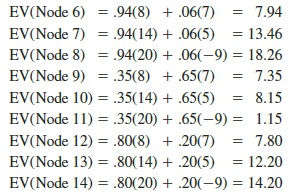
Figure 19.6 shows the reduced decision tree after computing expected values at these chance nodes.

Next move to decision nodes 3, 4, and 5. For each of these nodes, we select the decision alternative branch that leads to the best expected value. For example, at node 3 we have the choice of the small complex branch with EV(Node 6) = 7.94, the medium complex branch with EV(Node 7) = 13.46, and the large complex branch with EV(Node 8) = 18.26. Thus, we select the large complex decision alternative branch and the expected value at node 3 becomes EV(Node 3) = 18.26.

For node 4, we select the best expected value from nodes 9, 10, and 11. The best de­cision alternative is the medium complex branch that provides EV(Node 4) = 8.15. For node 5, we select the best expected value from nodes 12, 13, and 14. The best decision alternative is the large complex branch that provides EV(Node 5) = 14.20. Figure 19.7 shows the reduced decision tree after choosing the best decisions at nodes 3, 4, and 5.

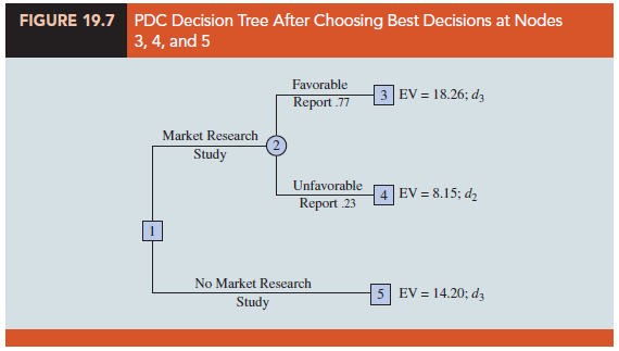
The expected value at chance node 2 can now be computed as follows:

EV(Node 2) = .77EV(Node 3) + .23EV(Node 4)

= .77(18.26) + .23(8.15) = 15.93

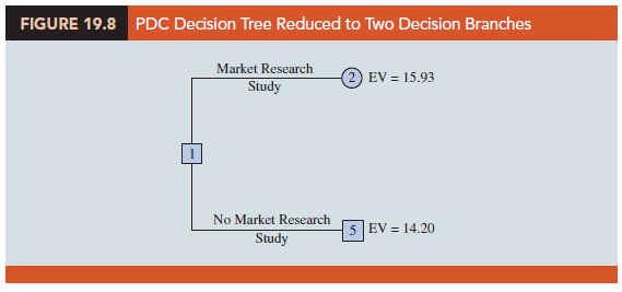
This calculation reduces the decision tree to one involving only the two decision branches from node 1 (see Figure 19.8).

Finally, the decision can be made at decision node 1 by selecting the best expected val­ues from nodes 2 and 5. This action leads to the decision alternative to conduct the market research study, which provides an overall expected value of 15.93.

The optimal decision for PDC is to conduct the market research study and then carry out the following decision strategy:

If the market research is favorable, construct the large condominium complex.

If the market research is unfavorable, construct the medium condominium complex.

The analysis of the PDC decision tree illustrates the methods that can be used to analyze more complex sequential decision problems. First, draw a decision tree consisting of decision and chance nodes and branches that describe the sequential nature of the problem. Determine the probabilities for all chance outcomes. Then, by working backward through the tree, compute expected values at all chance nodes and select the best decision branch at all decision nodes. The sequence of optimal decision branches determines the optimal decision strategy for the problem.

3. Expected Value of Sample Information

In the PDC problem, the market research study is the sample information used to determine the optimal decision strategy. The expected value associated with the market research study is $15.93. In Section 19.2 we showed that the best expected value if the market research study is not undertaken is $14.20. Thus, we can conclude that the difference, $15.93 – $14.20 = $1.73, is the expected value of sample information (EVSI). In other words, conducting the market research study adds $1.73 million to the PDC expected value. In general, the expected value of sample information is as follows:

Note the role of the absolute value in equation (19.5). For minimization problems the expected value with sample information is always less than or equal to the expected value without sample information. In this case, EVSI is the magnitude of the difference between EVwSI and EVwoSI; thus, by taking the absolute value of the difference as shown in equation (19.5), we can handle both the maximization and minimization cases with one equation.

Source:  Anderson David R., Sweeney Dennis J., Williams Thomas A. (2019), Statistics for Business & Economics, Cengage Learning; 14th edition.