The Social Costs of Monopoly Power

In a competitive market, price equals marginal cost. Monopoly power, on the other hand, implies that price exceeds marginal cost. Because monopoly power results in higher prices and lower quantities produced, we would expect it to make consumers worse off and the firm better off. But suppose we value the welfare of consumers the same as that of producers. In the aggregate, does monopoly power make consumers and producers better or worse off?

We can answer this question by comparing the consumer and producer sur- plus that results when a competitive industry produces a good with the surplus that results when a monopolist supplies the entire market.11  (We assume that the competitive market and the monopolist have the same cost curves.) Figure 10.10 shows the average and marginal revenue curves and marginal cost curve for the monopolist. To maximize profit, the firm produces at the point where marginal revenue equals marginal cost, so that the price and quantity are Pm  and Qm. In a competitive market, price must equal marginal cost, so the competitive price and quantity, Pc  and Qc  are found at the intersection of the average revenue (demand) curve and the marginal cost curve. Now let’s examine how surplus changes if we move from the competitive price and quantity, Pc  and Qc, to the monopoly price and quantity, Pm  and Qm.

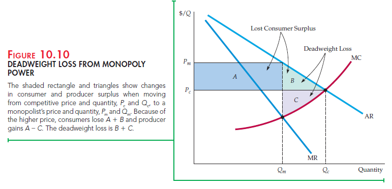
Under monopoly, the price is higher and consumers buy less. Because of the higher price, those consumers who buy the good lose surplus of an amount given by rectangle A. Those consumers who do not buy the good at price Pm  but who would buy at price Pc  also lose surplus—namely, an amount given by triangle B. The total loss of consumer surplus is therefore A + B. The producer, however, gains rectangle A by selling at the higher price but loses triangle C, the additional profit it would have earned by selling Qc  − Qm  at price Pc. The total gain in producer surplus is therefore A − C. Subtracting the loss of consumer surplus from the gain in producer surplus, we see a net loss of surplus given by B + C. This is the deadweight loss from monopoly power. Even if the monopolist’s profits were taxed away and redistributed to the consum- ers of its products, there would be an inefficiency because output would be lower than under conditions of competition. The deadweight loss is the social cost of this inefficiency.

1. Rent Seeking

In practice, the social cost of monopoly power is likely to exceed the dead- weight loss in triangles B and C of Figure 10.10. The reason is that the firm may engage in rent seeking: spending large amounts of money in socially unpro- ductive efforts to acquire, maintain, or exercise its monopoly power. Rent seeking might involve lobbying activities (and perhaps campaign contribu- tions) to obtain government regulations that make entry by potential competi- tors more difficult. Rent-seeking activity could also involve advertising and legal efforts to avoid antitrust scrutiny. It might also mean installing but not utilizing extra production capacity to convince potential competitors that they cannot sell enough to make entry worthwhile. We would expect the economic incentive to incur rent-seeking costs to bear a direct relation to the gains from monopoly power (i.e., rectangle A minus triangle C.) Therefore, the larger the transfer from consumers to the firm (rectangle A), the larger the social cost of monopoly.12

Here’s an example. In 1996, the Archer Daniels Midland Company (ADM) successfully lobbied the Clinton administration for regulations requiring that the ethanol (ethyl alcohol) used in motor vehicle fuel be produced from corn. (The government had already planned to add ethanol to gasoline in order to reduce the country’s dependence on imported oil.) Ethanol is chemically the same whether it is produced from corn, potatoes, grain, or anything else. Then why require that it be produced only from corn? Because ADM had a near monopoly on corn-based ethanol production, so the regulation would increase its gains from monopoly power.

2. Price Regulation

Because of its social cost, antitrust laws prevent firms from accumulating exces- sive amounts of monopoly power. We will say more about such laws at the end of the chapter. Here, we examine another means by which government can limit monopoly power—price regulation.

We saw in Chapter 9 that in a competitive market, price regulation always results in a deadweight loss. This need not be the case, however, when a firm has monopoly power. On the contrary, price regulation can eliminate the dead- weight loss that results from monopoly power.

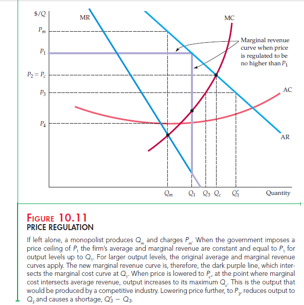
Figure 10.11 illustrates price regulation. Pm  and Qm  are the price and quantity that result without regulation—i.e., at the point where marginal revenue equals marginal cost. Now suppose the price is regulated to be no higher than P1. To find the firm’s profit-maximizing output, we must determine how its average and marginal revenue curves are affected by the regulation.

Because the firm can charge no more than P1  for output levels up to Q1, its new average revenue curve is a horizontal line at P1. For output levels greater than Q1, the new average revenue curve is identical to the old average revenue curve: At these output levels, the firm will charge less than P1  and so will be unaffected by the regulation.

The firm’s new marginal revenue curve corresponds to its new average rev- enue curve and is shown by the purple line in Figure 10.11. For output levels up to Q1, marginal revenue equals average revenue. (Recall that, as with a competi- tive firm, if average revenue is constant, average revenue and marginal revenue are equal.) For output levels greater than Q1, the new marginal revenue curve is identical to the original curve. Thus the complete marginal revenue curve now has three pieces: (1) the horizontal line at P1  for quantities up to Q1; (2) a verti- cal line at the quantity Q1  connecting the original average and marginal revenue curves; and (3) the original marginal revenue curve for quantities greater than Q1.

To maximize its profit, the firm should produce the quantity Q1  because that is the point at which its marginal revenue curve intersects its marginal cost curve. You can verify that at price P1 and quantity Q1, the deadweight loss from monopoly power is reduced.

As the price is lowered further, the quantity produced continues to increase and the deadweight loss to decline. At price Pc where average revenue and mar- ginal cost intersect, the quantity produced has increased to the competitive level; the deadweight loss from monopoly power has been eliminated. Reducing the price even more—say, to P3—results in a reduction in quantity. This reduction is equivalent to imposing a price ceiling on a competitive industry. A shortage develops, (Q=   – Q ), in addition to the deadweight loss from regulation. As the price is lowered further, the quantity produced continues to fall and the short- age grows. Finally, if the price is lowered below P4, the minimum average cost, the firm loses money and goes out of business.

3. Natural Monopoly

Price regulation is most often used for natural monopolies, such as local utility companies. A natural monopoly is a firm that can produce the entire output of the market at a cost that is lower than what it would be if there were several firms. If a firm is a natural monopoly, it is more efficient to let it serve the entire market rather than have several firms compete.

A natural monopoly usually arises when there are strong economies of scale, as illustrated in Figure 10.12. If the firm represented by the figure was broken up into two competing firms, each supplying half the market, the average cost for each would be higher than the cost incurred by the original monopoly.

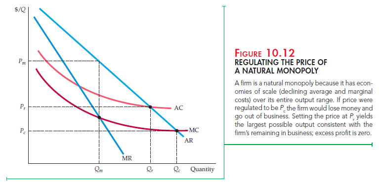
Note in Figure 10.12 that because average cost is declining everywhere, mar- ginal cost is always below average cost. If the firm were unregulated, it would produce Qm  and sell at the price Pm. Ideally, the regulatory agency would like to push the firm’s price down to the competitive level Pc. At that level, however, price would not cover average cost and the firm would go out of business. The best alternative is therefore to set the price at Pr, where average cost and average revenue intersect. In that case, the firm earns no monopoly profit, while output remains as large as possible without driving the firm out of business.

4. Regulation in Practice

Recall that the competitive price (Pc  in Figure 10.11) is found at the point at which the firm’s marginal cost and average revenue (demand) curves intersect. Likewise for a natural monopoly: The minimum feasible price (Pr in Figure 10.12) is found at the point at which average cost and demand intersect. Unfortunately, it is often difficult to determine these prices accurately in practice because the firm’s demand and cost curves may shift as market conditions evolve.

As a result, the regulation of a monopoly is sometimes based on the rate of return that it earns on its capital. The regulatory agency determines an allowed price, so that this rate of return is in some sense “competitive” or “fair.” This practice is called rate-of-return regulation: The maximum price allowed is based on the (expected) rate of return that the firm will earn.13

Unfortunately, difficult problems arise when implementing rate-of-return regulation. First, although it is a key element in determining the firm’s rate of return, a firm’s capital stock is difficult to value. Second, while a “fair” rate of return must be based on the firm’s actual cost of capital, that cost depends in turn on the behavior of the regulatory agency (and on investors’ perceptions of what allowed rates of return will be in the future).

The difficulty of agreeing on a set of numbers to be used in rate-of-return calculations often leads to delays in the regulatory response to changes in cost and other market conditions (not to mention long and expensive regula- tory hearings). The major beneficiaries are usually lawyers, accountants, and, occasionally, economic consultants. The net result is regulatory lag—the delays of a year or more usually entailed in changing regulated prices.

Another approach to regulation is setting price caps based on the firm’s vari- able costs, past prices, and possibly inflation and productivity growth. A price cap can allow for more flexibility than rate-of-return regulation. Under price cap regulation, for example, a firm would typically be allowed to raise its prices each year (without having to get approval from the regulatory agency) by an amount equal to the actual rate of inflation, minus expected productivity growth. Price cap regulation of this sort has been used to control prices of long distance and local telephone service.

By the 1990s, the regulatory environment in the United States had changed dramatically. Many parts of the telecommunications industry had been dereg- ulated, as had electric utilities in many states. Because scale economies had been largely exhausted, there was no reason to regard these firms as natu- ral monopolies. In addition, technological change made entry by new firms relatively easy.

Source: Pindyck Robert, Rubinfeld Daniel (2012), Microeconomics, Pearson, 8th edition.