How to Use Bootstrapping to Account for Non-Normal Data in SEM

One of the fundamental assumptions with SEM is that your data is normally distributed. Having non-normal data can lead to chi-square values being inflated and thus can lead researchers to start making changes or alterations in a model that are not really needed. To address the issue of having non-normal data, you can look for multivariate outliers, and this might address your issues in a small sample.The best and most frequently used technique to address non-normality is to use a bootstrap in the analysis. In the mediation discussion in Chapter 6, I go into detail about what is a bootstrap and how it is performed for mediation testing.We are going to use a very similar process here in using bootstrapping to assess a model with non-normal data.

After you have formed your model in AMOS and determined that your data is non-normal (see page 165), you need to run your analysis with a bootstrap sample. To accomplish this, you will go into the Analysis Properties window and then select the Bootstrap tab at the top. You will need to select the option that says “Perform bootstrap”.You will need to change the number of samples from 200 to 5,000. Having a sample of 5,000 is sufficiently large to achieve stability in the results. You will then select the “Bias-corrected confidence intervals” option and change the confidence interval from 90 to 95. Next, you will need to select the option “Bootstrap ML” in order to run the bootstrap via maximum likelihood. After those options are checked, you are ready to run the analysis again.

Figure 10.7  Performing ML Bootstrap in Analysis Properties Window

Let’s use our full structural model example from Chapter 5 and assume our data is not normally distributed. This example states that Adaptive Behavior and Servicescape is going to positively influence Customer Delight feelings, which are going to positively influence the dependent variables of Tolerance to Future Failures and Intentions to Spread Positive Word of Mouth.

Figure 10.8 Full Structural Model in AMOS to Test Non-Normal Data

After drawing the model and selecting the bootstrapping options just detailed, you are ready to run your analysis. In the output, go to the “Estimates” link and you will see the unstandardized and standardized estimates of your model. This is information we will need, but we also need to find the bootstrap estimates for each hypothesized relationship.

Figure 10.9 Estimates Output of Regression Weights in Full Structural Model

After viewing the “Estimates” link, you need to go to the “Scalars” link and then select “Regression Weights”. This will initially just show you the unstandardized estimates that you just saw in the “Estimates” link. After you have selected the “Regression Weights” link, there should be additional links that become available at the bottom left part of the page.These links are “Bootstrap errors” and “Bias-corrected percentile method”. Select the “Bias-corrected per- centile method”.This link will present the unstandardized regression estimates, but it will also present a bootstrap confidence interval for each estimate.The bootstrap estimate will let you know if your unstandardized estimates fall within the 95% confidence interval when 5,000 bootstrap samples were used to “normalize” the data.

Figure 10.10 Unstandardized Regression Weights With Confidence Intervals Based on Bootstrap

In this example, all estimates fall within a confidence interval that does not include zero. You can also see a p-value for each bootstrap confidence interval. Thus, we can conclude that our estimates are valid based on the bootstrapping technique to normalize the data.

One of the primary concerns with non-normal data is the inflation of model fit estimates.To assess model fit with the bootstrap samples, we are going to use to the Bollen-Stine method. This method will allow us to see if the proposed model fits the data when the bootstrap sam- ples are used as the input. AMOS can be a little quirky when asking for a Bollen-Stine boot- strap. If we simply ask for the Bollen-Stine option in Analysis Properties when “Bias-corrected confidence interval” is selected, AMOS will not produce the estimate. If you select the Bollen- Stine bootstrap, you have to uncheck the “Bias-corrected confidence interval” option. Thus, I run the bootstrap initially with the Bias-corrected confidence intervals and get the informa- tion I need, and then I run a separate analysis for the Bollen-Stine bootstrap with the Bias- corrected confidence intervals option not checked.

Figure 10.11  Selecting Bollen-Stine Bootstrap in Analysis Properties Window

After selecting the Bollen-Stine option and running the analysis again, let’s initially examine the model fit estimates in the output. We can see that the model fit for our model has a chi- square value of 225.34 with 130 degrees of freedom.

Figure 10.12 Model Fit Statistics in AMOS

If we select the Bootstrap distributions link on the left-hand side, we can see the distribu- tion of chi-square values across the 5,000 bootstrap samples that were run with the proposed model.You can see the mean value was 188.04 and that our initial chi-square value of 225.34 is clearly within the distribution that ranges from 91.35 to 366.43.

Figure 10.13  Bootstrap Distribution of Chi-Square Values

Next, we need to examine the Bollen-Stine bootstrap which is accessed via a separate link above the Bootstrap distributions option. Clicking on this link will bring up the Bollen- Stine test results. The Bollen-Stine test will initially tell you how many bootstrap samples fit the model better than the initial estimate, and it will also tell you how many samples fit equally well or actually fit worse. Your goal is to have a Bollen-Stine bootstrap that is non-significant because this means the model still has an adequate “fit” with the bootstrap samples. If you have a significant Bollen-Stine estimate, then it states your model fit is problematic based on the bootstrap estimates that are trying to “normalize” the data. In this example, 4,300 samples fit better, 700 samples fit worse, and the Bollen-Stine estimate was a p-value of .14. Thus, we can conclude that the model still has an adequate fit with the bootstrap samples.

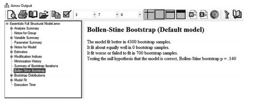
Figure 10.14  Bollen-Stine Bootstrap Results in AMOS

If the Bollen-Stine bootstrap is rejected (found a significant result p < .05), this should give the researcher pause in moving forward because the result means the model is not fitting the data. Saying that, the Bollen-Stine is very sensitive to sample size, and it is advisable to use numerous goodness (and badness) of fit indices to determine model fit. Bollen-Stine accesses only chi-square values, but it is always advisable to use numerous different model fit options in presenting results.

Source: Thakkar, J.J. (2020). “Procedural Steps in Structural Equation Modelling”. In: Structural Equation Modelling. Studies in Systems, Decision and Control, vol 285. Springer, Singapore.