Over time, fixed assets, with the exception of land, lose their ability to provide services. Thus, the costs of fixed assets such as equipment and buildings should be recorded as an expense over their useful lives. This periodic recording of the cost of fixed assets as an expense is called depreciation. Because land has an unlimited life, it is not depreciated.
The adjusting entry to record depreciation debits Depreciation Expense and credits a contra asset account entitled Accumulated Depreciation or Allowance for Depreciation. The use of a contra asset account allows the original cost to remain unchanged in the fixed asset account.
Depreciation can be caused by physical or functional factors.
- Physical depreciation factors include wear and tear during use or from exposure to weather.
- Functional depreciation factors include obsolescence and changes in customer needs that cause the asset to no longer provide services for which it was intended. For example, equipment may become obsolete due to changing technology.
Two common misunderstandings that exist about depreciation as used in accounting include:
- Depreciation does not measure a decline in the market value of a fixed asset. Instead, depreciation is an allocation of a fixed asset’s cost to expense over the asset’s useful life. Thus, the book value of a fixed asset (cost less accumulated depreciation) usually does not agree with the asset’s market value. This is justified in accounting because a fixed asset is for use in a company’s operations rather than for resale.
- Depreciation does not provide cash to replace fixed assets as they wear out. This misunderstanding may occur because depreciation, unlike most expenses, does not require an outlay of cash when it is recorded.
1. Factors in Computing Depreciation Expense
Three factors determine the depreciation expense for a fixed asset. These three factors are as follows:
- The asset’s initial cost
- The asset’s expected useful life
- The asset’s estimated residual value
The initial cost of a fixed asset is determined using the concepts discussed and illustrated earlier in this chapter.
The expected useful life of a fixed asset is estimated at the time the asset is placed into service. Estimates of expected useful lives are available from industry trade associations. The Internal Revenue Service also publishes guidelines for useful lives, which may be helpful for financial reporting purposes. However, it is not uncommon for different companies to use a different useful life for similar assets.
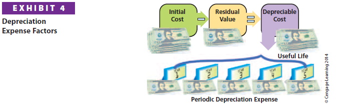
The residual value of a fixed asset at the end of its useful life is estimated at the time the asset is placed into service. Residual value is sometimes referred to as scrap value, salvage value, or trade-in value. The difference between a fixed asset’s initial cost and its residual value is called the asset’s depreciable cost. The depreciable cost is the amount of the asset’s cost that is allocated over its useful life as depreciation expense. If a fixed asset has no residual value, then its entire cost should be allocated to depreciation.
Exhibit 4 shows the relationship between depreciation expense and a fixed asset’s initial cost, expected useful life, and estimated residual value.
For an asset placed into or taken out of service during the first half of a month, many companies compute depreciation on the asset for the entire month. That is, the asset is treated as having been purchased or sold on the first day of that month. Likewise, purchases and sales during the second half of a month are treated as having occurred on the first day of the next month. To simplify, this practice is used in this chapter.
The three depreciation methods used most often are as follows:[1]
- Straight-line depreciation
- Units-of-output depreciation
- Double-declining-balance depreciation
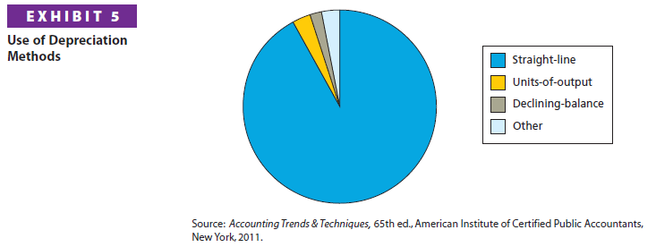
Exhibit 5 shows how often these methods are used in financial statements.
It is not necessary for a company to use only one method of computing depreciation for all of its fixed assets. For example, a company may use one method for depreciating equipment and another method for depreciating buildings.
A company may also use different depreciation methods for determining income taxes and property taxes.
2. Straight-Line Method
The straight-line method provides for the same amount of depreciation expense for each year of the asset’s useful life. As shown in Exhibit 5, the straight-line method is by far the most widely used depreciation method.
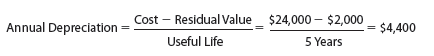
To illustrate, assume that equipment was purchased on January 1 as follows:
Initial cost $24,000
Expected useful life 5 years
Estimated residual value $2,000
The annual straight-line depreciation of $4,400 is computed below.
If an asset is used for only part of a year, the annual depreciation is prorated. For example, assume that the preceding equipment was purchased and placed into service on October 1. The depreciation for the year ending December 31 would be $1,100, computed as follows:
First-Year Partial Depreciation = $4,400 X 3/12 = $1,100
The computation of straight-line depreciation may be simplified by converting the annual depreciation to a percentage of depreciable cost.3 The straight-line percentage is determined by dividing 100% by the number of years of expected useful life, as shown below.
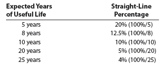
For the preceding equipment, the annual depreciation of $4,400 can be computed by multiplying the depreciable cost of $22,000 by 20% (100%/5).
As shown on the previous page, the straight-line method is simple to use. When an asset’s revenues are about the same from period to period, straight-line depreciation provides a good matching of depreciation expense with the asset’s revenues.
3. Units-of-Output Method
The units-of-output method provides the same amount of depreciation expense for each unit of output of the asset. Depending on the asset, the units of output can be expressed in terms of hours, miles driven, or quantity produced. For example, the unit of output for a truck is normally expressed in miles driven. For manufacturing assets, the units of output are often expressed as units of product. In this case, the units-of-output method may be called the units-of-production method.
The units-of-output method is applied in two steps.
Step 1. Determine the depreciation per unit as:
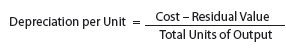
Step 2. Compute the depreciation expense as:
Depreciation Expense = Depreciation per Unit x Total Units of Output Used
To illustrate, assume that the equipment in the preceding example is expected to have a useful life of 10,000 operating hours. During the year, the equipment was operated 2,100 hours. The units-of-output depreciation for the year is $4,620, as shown below.
Step 1. Determine the depreciation per hour as:
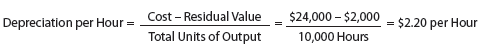
Step 2. Compute the depreciation expense as:
Depreciation Expense = Depreciation per Unit x Total Units of Output Used
Depreciation Expense = $2.20 per Hour x 2,100 Hours = $4,620
The units-of-output method is often used when a fixed asset’s in-service time (or use) varies from year to year. In such cases, the units-of-output method matches depreciation expense with the asset’s revenues.
4. Double-Declining-Balance Method
The double-declining-balance method provides for a declining periodic expense over the expected useful life of the asset. The double-declining-balance method is applied in three steps.
Step 1. Determine the straight-line percentage, using the expected useful life.
Step 2. Determine the double-declining-balance rate by multiplying the straightline rate from Step 1 by 2.
Step 3. Compute the depreciation expense by multiplying the double-declining- balance rate from Step 2 times the book value of the asset.
To illustrate, the equipment purchased in the preceding example is used to compute double-declining-balance depreciation. For the first year, the depreciation is $9,600, as shown below.
Step 1. Straight-line percentage = 20% (100%/5)
Step 2. Double-declining-balance rate = 40% (20% X 2)
Step 3. Depreciation expense = $9,600 ($24,000 X 40%)
For the first year, the book value of the equipment is its initial cost of $24,000. After the first year, the book value (cost minus accumulated depreciation) declines and, thus, the depreciation also declines. The double-declining-balance depreciation for the full five-year life of the equipment is shown below.
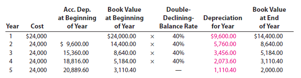
When the double-declining-balance method is used, the estimated residual value is not considered. However, the asset should not be depreciated below its estimated residual value. In the above example, the estimated residual value was $2,000. Therefore, the depreciation for the fifth year is $1,110.40 ($3,110.40 – $2,000.00) instead of $1,244.16 (40% X $3,110.40).
Like straight-line depreciation, if an asset is used for only part of a year, the annual depreciation is prorated. For example, assume that the preceding equipment was purchased and placed into service on October 1. The depreciation for the year ending December 31 would be $2,400, computed as follows:
First-Year Partial Depreciation = $9,600 x 3/12 = $2,400
The depreciation for the second year would then be $8,640, computed as follows:
Second-Year Depreciation = $8,640 = [40% x ($24,000 – $2,400)]
The double-declining-balance method provides a higher depreciation in the first year of the asset’s use, followed by declining depreciation amounts. For this reason, the double-declining-balance method is called an accelerated depreciation method.
An asset’s revenues are often greater in the early years of its use than in later years. In such cases, the double-declining-balance method provides a good matching of depreciation expense with the asset’s revenues.
5. Comparing Depreciation Methods
The three depreciation methods are summarized in Exhibit 6. All three methods allocate a portion of the total cost of an asset to an accounting period, while never depreciating an asset below its residual value.
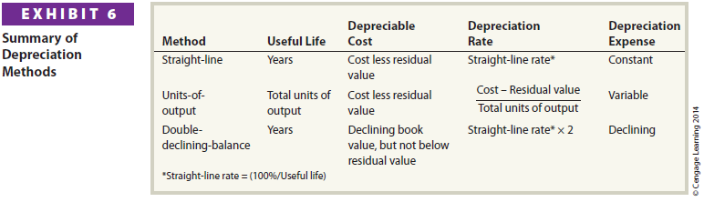
The straight-line method provides for the same periodic amounts of depreciation expense over the life of the asset. The units-of-output method provides for periodic amounts of depreciation expense that vary, depending on the amount the asset is used. The double-declining-balance method provides for a higher depreciation amount in the first year of the asset’s use, followed by declining amounts.
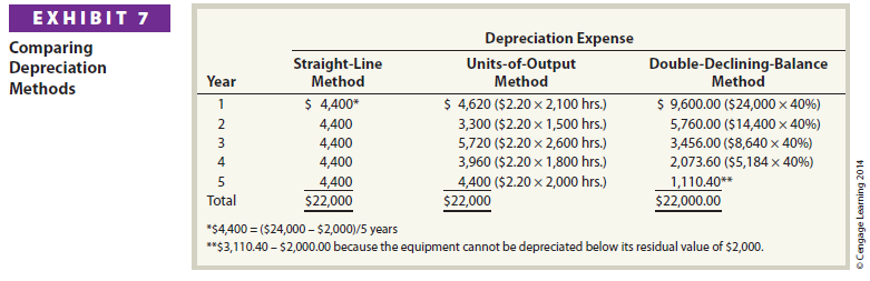
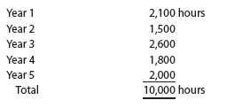
The depreciation for the straight-line, units-of-output, and double-decliningbalance methods is shown in Exhibit 7. The depreciation in Exhibit 7 is based on the equipment purchased in our prior illustrations. For the units-of-output method, we assume that the equipment was used as follows:
6. Depreciation for Federal Income Tax
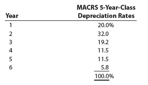
The Internal Revenue Code uses the Modified Accelerated Cost Recovery System (MACRS) to compute depreciation for tax purposes. MACRS has eight classes of useful life and depreciation rates for each class. Two of the most common classes are the five-year class and the seven-year class.4 The five-year class includes automobiles and light-duty trucks. The seven-year class includes most machinery and equipment. Depreciation for these two classes is similar to that computed using the doubledeclining-balance method.
In using the MACRS rates, residual value is ignored. Also, all fixed assets are assumed to be put in and taken out of service in the middle of the year. For the fiveyear-class assets, depreciation is spread over six years, as shown below.
To simplify, a company will sometimes use MACRS for both financial statement and tax purposes. This is acceptable if MACRS does not result in significantly different amounts than would have been reported using one of the three depreciation methods discussed in this chapter.
7. Revising Depreciation Estimates
Estimates of residual values and useful lives of fixed assets may change due to abnormal wear and tear or obsolescence. When new estimates are determined, they are used to determine the depreciation expense in future periods. The depreciation expense recorded in earlier years is not affected.5
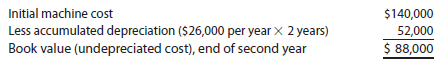
To illustrate, assume the following data for a machine that was purchased on January 1, 2013:
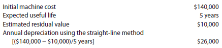
At the end of 2014, the machine’s book value (undepreciated cost) is $88,000, as shown below.
At the beginning of 2015, the company estimates that the machine’s remaining useful life is eight years (instead of three) and that its residual value is $8,000 (instead of $10,000). The depreciation expense for each of the remaining eight years is $10,000, computed as follows:
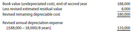
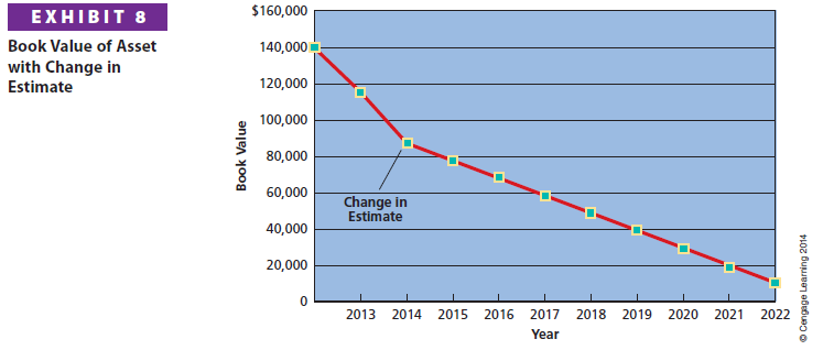
Exhibit 8 shows the book value of the asset over its original and revised lives. After the depreciation is revised at the end of 2014, book value declines at a slower rate. At the end of year 2022, the book value reaches the revised residual value of $8,000.
Source: Warren Carl S., Reeve James M., Duchac Jonathan (2013), Corporate Financial Accounting, South-Western College Pub; 12th edition.
Hello there, I discovered your web site by the use of Google whilst looking for a related subject, your site came up, it appears to be like good. I have bookmarked it in my google bookmarks.