As an example of an experimental statistical study, let us consider the problem facing Chemitech, Inc. Chemitech developed a new filtration system for municipal water supplies. The components for the new filtration system will be purchased from several suppliers, and Chemitech will assemble the components at its plant in Columbia, South Carolina.
The industrial engineering group is responsible for determining the best assembly method for the new filtration system. After considering a variety of possible approaches, the group narrows the alternatives to three: method A, method B, and method C. These methods differ in the sequence of steps used to assemble the system. Managers at Chemitech want to determine which assembly method can produce the greatest number of filtration systems per week.
In the Chemitech experiment, assembly method is the independent variable or factor. Because three assembly methods correspond to this factor, we say that three treatments are associated with this experiment; each treatment corresponds to one of the three assembly methods. The Chemitech problem is an example of a single-factor experiment; it involves one categorical factor (method of assembly). More complex experiments may consist of multiple factors; some factors may be categorical and others may be quantitative.
The three assembly methods or treatments define the three populations of interest for the Chemitech experiment. One population is all Chemitech employees who use assembly method A, another is those who use method B, and the third is those who use method C. Note that for each population the dependent or response variable is the number of filtration systems assembled per week, and the primary statistical objective of the experiment is to determine whether the mean number of units produced per week is the same for all three populations (methods).
Suppose a random sample of three employees is selected from all assembly workers at the Chemitech production facility. In experimental design terminology, the three randomly selected workers are the experimental units. The experimental design that we will use for the Chemitech problem is called a completely randomized design. This type of design requires that each of the three assembly methods or treatments be assigned randomly to one of the experimental units or workers. For example, method A might be randomly assigned to the second worker, method B to the first worker, and method C to the third worker. The concept of randomization, as illustrated in this example, is an important principle of all experimental designs.
Note that this experiment would result in only one measurement or number of units assembled for each treatment. To obtain additional data for each assembly method, we must repeat or replicate the basic experimental process. Suppose, for example, that instead of selecting just three workers at random we selected 15 workers and then randomly assigned each of the three treatments to 5 of the workers. Because each method of assembly is assigned to 5 workers, we say that five replicates have been obtained. The process of replication is another important principle of experimental design. Figure 13.1 shows the completely randomized design for the Chemitech experiment.

1. Data Collection
Once we are satisfied with the experimental design, we proceed by collecting and analyzing the data. In the Chemitech case, the employees would be instructed in how to perform the assembly method assigned to them and then would begin assembling the new filtration systems using that method. After this assignment and training, the number of units assembled by each employee during one week is as shown in Table 13.1. The sample means, sample variances, and sample standard deviations for each assembly method are also provided. Thus, the sample mean number of units produced using method A is 62; the sample mean using method B is 66; and the sample mean using method C is 52. From these data, method B appears to result in higher production rates than either of the other methods.

The real issue is whether the three sample means observed are different enough for us to conclude that the means of the populations corresponding to the three methods of assembly are different. To write this question in statistical terms, we introduce the following notation.
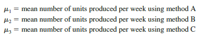
Although we will never know the actual values of m1, m2, and m3, we want to use the sample means to test the following hypotheses.
As we will demonstrate shortly, analysis of variance (ANOVA) is the statistical procedure used to determine whether the observed differences in the three sample means are large enough to reject H0.
2. Assumptions for Analysis of Variance
Three assumptions are required to use analysis of variance.
- For each population, the response variable is normally distributed. Implication: In the Chemitech experiment, the number of units produced per week (response variable) must be normally distributed for each assembly method.
- The variance of the response variable, denoted s2, is the same for all of the populations. Implication: In the Chemitech experiment, the variance of the number of units produced per week must be the same for each assembly method.
- The observations must be independent. Implication: In the Chemitech experiment, the number of units produced per week for each employee must be independent of the number of units produced per week for any other employee.
3. Analysis of Variance: A Conceptual Overview
If the means for the three populations are equal, we would expect the three sample means to be close together. In fact, the closer the three sample means are to one another, the weaker the evidence we have for the conclusion that the population means differ. Alternatively, the more the sample means differ, the stronger the evidence we have for the conclusion that the population means differ. In other words, if the variability among the sample means is “small,” it supports H0; if the variability among the sample means is “large,” it supports Ha.
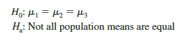
If the null hypothesis, H0: m1 = m2 = m3, is true, we can use the variability among the sample means to develop an estimate of s2. First, note that if the assumptions for analysis of variance are satisfied and the null hypothesis is true, each sample will have come from the same normal distribution with mean m and variance s2. Recall from Chapter 7 that the sampling distribution of the sample mean x for a simple random sample of size n from a normal population will be normally distributed with mean m and variance s2/n. Figure 13.2 illustrates such a sampling distribution.
Thus, if the null hypothesis is true, we can think of each of the three sample means,
X1 = 62, X2 = 66, and X3 = 52 from Table 13.1, as values drawn at random from the sampling distribution shown in Figure 13.2. In this case, the mean and variance of the three X values can be used to estimate the mean and variance of the sampling distribution. When the sample sizes are equal, as in the Chemitech experiment, the best estimate of the mean of the sampling distribution of X is the mean or average of the sample means. In the Chemitech experiment, an estimate of the mean of the sampling distribution of X is (62 + 66 + 52)/3 = 60. We refer to this estimate as the overall sample mean. An estimate of the variance of the sampling distribution of X, σ 2x, is provided by the variance of the three sample means.

The result, ns2 x= 260, is referred to as the between-treatments estimate of σ2.
The between-treatments estimate of σ2 is based on the assumption that the null hypothesis is true. In this case, each sample comes from the same population, and there is only one sampling distribution of X. To illustrate what happens when H0 is false, suppose the population means all differ. Note that because the three samples are from normal populations with different means, they will result in three different sampling distributions. Figure 13.3 shows that in this case, the sample means are not as close together as they were when H0 was true. Thus, s2x will be larger, causing the between-treatments estimate of σ2 to be larger. In general, when the population means are not equal, the between-treatments estimate will overestimate the population variance σ2.

The variation within each of the samples also has an effect on the conclusion we reach in analysis of variance. When a simple random sample is selected from each population, each of the sample variances provides an unbiased estimate of a2. Hence, we can combine or pool the individual estimates of a2 into one overall estimate. The estimate of a2 obtained in this way is called the pooled or within-treatments estimate of a2. Because each sample variance provides an estimate of a2 based only on the variation within each sample, the within-treatments estimate of a2 is not affected by whether the population means are equal. When the sample sizes are equal, the within-treatments estimate of a2 can be obtained by computing the average of the individual sample variances. For the Chemitech experiment we obtain

In the Chemitech experiment, the between-treatments estimate of σ2 (260) is much larger than the within-treatments estimate of σ2 (28.33). In fact, the ratio of these two estimates is 260/28.33 = 9.18. Recall, however, that the between-treatments approach provides a good estimate of σ2 only if the null hypothesis is true; if the null hypothesis is false, the between-treatments approach overestimates σ2. The within-treatments approach provides a good estimate of σ2 in either case. Thus, if the null hypothesis is true, the two estimates will be similar and their ratio will be close to 1. If the null hypothesis is false, the between-treatments estimate will be larger than the within-treatments estimate, and their ratio will be large. In the next section we will show how large this ratio must be to reject H0.
In summary, the logic behind ANOVA is based on the development of two independent estimates of the common population variance σ2. One estimate of σ2 is based on the variability among the sample means themselves, and the other estimate of σ2 is based on the variability of the data within each sample. By comparing these two estimates of σ2, we will be able to determine whether the population means are equal.
Source: Anderson David R., Sweeney Dennis J., Williams Thomas A. (2019), Statistics for Business & Economics, Cengage Learning; 14th edition.
You made some clear points there. I did a search on the issue and found most individuals will go along with with your site.