Trend Projection with Time Series Analysis

We present two forecasting methods in this section that are appropriate for time series exhibiting a trend pattern. First, we show how simple linear regression can be used to forecast a time series with a linear trend. Next we show how the curve-fitting capability of regression analysis can also be used to forecast time series with a curvilinear or nonlinear trend.

1. Linear Trend Regression

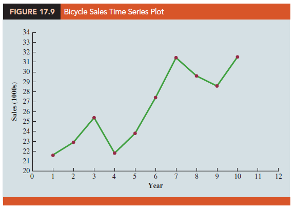
In Section 17.1 we used the bicycle sales time series in Table 17.3 and Figure 17.3 to illustrate a time series with a trend pattern. Let us now use this time series to illustrate how simple linear regression can be used to forecast a time series with a linear trend. The data for the bicycle time series are repeated in Table 17.12 and Figure 17.9.

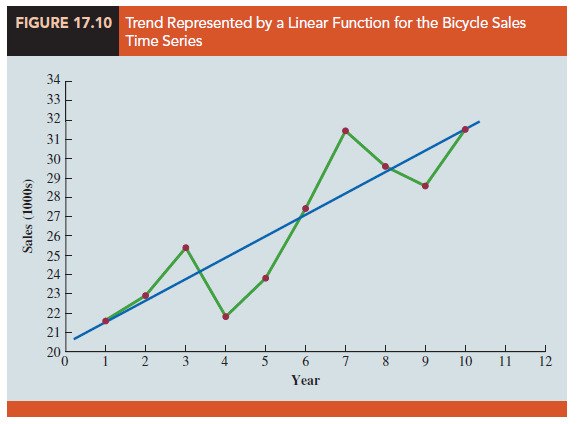
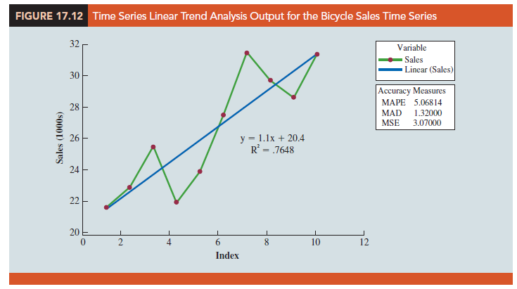
Although the time series plot in Figure 17.9 shows some up and down movement over the past 10 years, we might agree that the linear trend line shown in Figure 17.10 provides a reasonable approximation of the long-run movement in the series. We can use the methods of simple linear regression to develop such a linear trend line for the bicycle sales time series.

The estimated regression equation describing a straight-line relationship between an independent variable x and a dependent variable y is written as

where y is the estimated or predicted value of y. To emphasize the fact that in forecasting the independent variable is time, we will replace x with t and y with T_t to emphasize that we are estimating the trend for a time series. Thus, for estimating the linear trend in a time series we will use the following estimated regression equation.

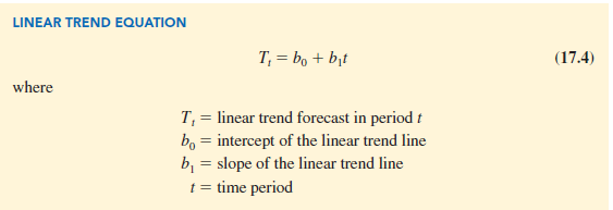
In equation (17.4), the time variable begins at t = 1 corresponding to the first time series observation (year 1 for the bicycle sales time series) and continues until t = n corresponding to the most recent time series observation (year 10 for the bicycle sales time series).

Thus, for the bicycle sales time series t = 1 corresponds to the oldest time series value and t = 10 corresponds to the most recent year. Formulas for computing the estimated regression coefficients (b1 and b0) in equation (17.4) follow.

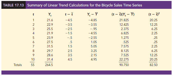
To compute the linear trend equation for the bicycle sales time series, we begin the calculations by computing t and Y using the information in Table 17.12.

Using these values, and the information in Table 17.13, we can compute the slope and intercept of the trend line for the bicycle sales time series.

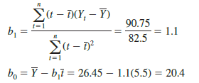
Therefore, the linear trend equation is

T_t = 20.4 + 1.1t

The slope of 1.1 indicates that over the past 10 years the firm experienced an average growth in sales of about 1100 units per year. If we assume that the past 10-year trend in sales is a good indicator of the future, this trend equation can be used to develop forecasts for future time periods. For example, substituting t = 11 into the equation yields next year’s trend projection or forecast, T₁₁.

T₁₁ = 20.4 + 1.1(11) = 32.5

Thus, using trend projection, we would forecast sales of 32,500 bicycles next year.

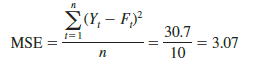
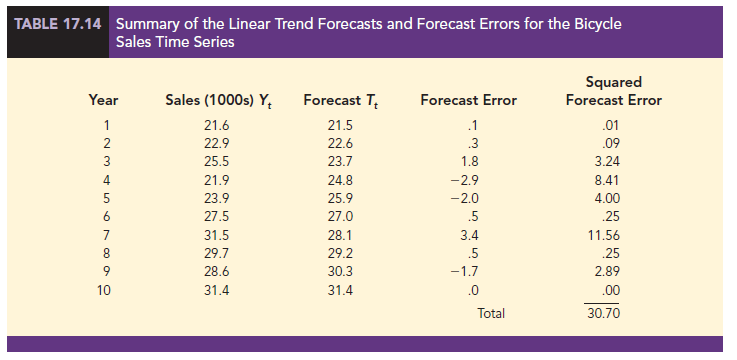
To compute the accuracy associated with the trend projection forecasting method, we will use the MSE. Table 17.14 shows the computation of the sum of squared errors for the bicycle sales time series. Thus, for the bicycle sales time series,

Because linear trend regression in forecasting is the same as the standard regression analysis procedure applied to time-series data, we can use statistical software to perform the calculations. Figure 17.11 shows a portion of the computer output for the bicycle sales time series.

In Figure 17.11 the value of MSE in the ANOVA table is

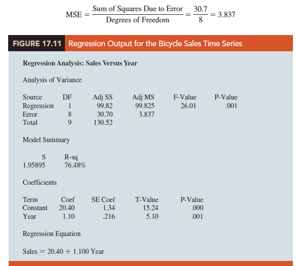
This value of MSE differs from the value of MSE that we computed previously because the sum of squared errors is divided by 8 instead of 10; thus, MSE in the regression output is not the average of the squared forecast errors. Most forecast­ing packages, however, compute MSE by taking the average of the squared errors. Thus, when using time series packages to develop a trend equation, the value of MSE that is reported may differ slightly from the value you would obtain using a general regression approach.

2. Nonlinear Trend Regression

The use of a linear function to model trend is common. However, as we discussed previously, sometimes time series have a curvilinear or nonlinear trend. As an example, consider the annual revenue in millions of dollars for a cholesterol drug for the first 10 years of sales. Table 17.15 shows the time series and Figure 17.13 shows the corre­sponding time series plot. For instance, revenue in year 1 was $23.1 million; revenue in year 2 was $21.3 million; and so on. The time series plot indicates an overall increasing or upward trend. But, unlike the bicycle sales time series, a linear trend does not appear to be appropriate. Instead, a curvilinear function appears to be needed to model the long-term trend.

Quadratic Trend Equation A variety of nonlinear functions can be used to develop an estimate of the trend for the cholesterol time series. For instance, consider the following quadratic trend equation:

For the cholesterol time series, t = 1 corresponds to year 1, t = 2 corresponds to year 2, and so on.

A standard linear regression procedure can be used to compute the values of b₀, b₁, and b₂. There are two independent variables, year and year squared, and the dependent variable is the sales revenue in millions of dollars. Thus, the first observation is 1, 1, 23.1; the second observation is 2, 4, 21.3; the third observation is 3, 9, 27.4; and so on. Figure 17.14 shows a portion of the multiple regression output for the quadratic trend model; the estimated regres­sion equation is

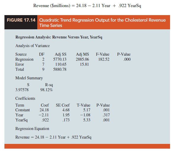
where

Year = 1, 2, 3,… , 10
YearSq = 1, 4, 9,… , 100

Using the standard multiple regression procedure requires us to compute the values for year squared as a second independent variable.

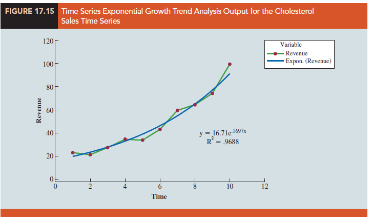
Exponential Trend Equation Another alternative that can be used to model the nonlinear pattern exhibited by the cholesterol time series is to fit an exponential model to the data. For instance, consider the following exponential trend equation:

To better understand this exponential trend equation, suppose b₀ = 16.71 and b₁ = .1697. Then, for t = 1, T₁ = 16.71 e ^1697(1) = 19.80; for t = 2, T₂ = 16.71 e ^1697(2) = 23.46; for t = 3, T₃ = 16.71 e^1697(3) = 27.80, and so forth for higher values of t. Note that T_t is not increasing by a constant amount as in the case of the linear trend model but by a constant percentage. In this exponential trend model, multiplicative factor is e ^1697(1) = 1.185, so the constant percentage increase from time period to time period is 18.5%.

Many statistical software packages have the capability to compute an exponential trend equation directly. Some software packages only provide linear trend, but by applying a natural log transformation to both sides of the equality in equation (17.8) we can apply the equivalent linear form:

Figure 17.15 shows the graphical output of an exponential trend equation based on equation (17.8) for the Cholesterol sales data.

Source:  Anderson David R., Sweeney Dennis J., Williams Thomas A. (2019), Statistics for Business & Economics, Cengage Learning; 14th edition.