In simple linear regression, we showed that the total sum of squares can be partitioned into two components: the sum of squares due to regression and the sum of squares due to error.
The same procedure applies to the sum of squares in multiple regression.
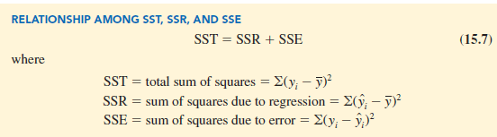
Because of the computational difficulty in computing the three sums of squares, we rely on computer packages to determine those values. The analysis of variance part of the output in Figure 15.4 shows the three values for the Butler Trucking problem with two independent variables: SST = 23.900, SSR = 21.6006, and SSE = 2.2994. With only one independent variable (number of miles traveled), the output in Figure 15.3 shows that SST = 23.900, SSR = 15.871, and SSE = 8.029. The value of SST is the same in both cases because it does not depend on y, but SSR increases and SSE decreases when a second independent variable (number of deliveries) is added. The implication is that the estimated multiple regression equation provides a better fit for the observed data.
In Chapter 14, we used the coefficient of determination, r2 = SSR/SST, to measure the goodness of fit for the estimated regression equation. The same concept applies to multiple regression. The term multiple coefficient of determination indicates that we are measuring the goodness of fit for the estimated multiple regression equation. The multiple coefficient of determination, denoted R2, is computed as follows:

The multiple coefficient of determination can be interpreted as the proportion of the variability in the dependent variable that can be explained by the estimated multiple regression equation. Hence, when multiplied by 100, it can be interpreted as the percentage of the variability in y that can be explained by the estimated regression equation.
In the two-independent-variable Butler Trucking example, with SSR = 21.6006 and SST = 23.900, we have
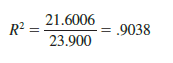
Therefore, 90.38% of the variability in travel time y is explained by the estimated multiple regression equation with miles traveled and number of deliveries as the independent variables. In Figure 15.4, we see that the multiple coefficient of determination (expressed as a percentage) is also provided; it is denoted by R-sq = 90.38%.
Figure 15.3 shows that the R-sq value for the estimated regression equation with only one independent variable, number of miles traveled (x^, is 66.41%. Thus, the percentage of the variability in travel times that is explained by the estimated regression equation increases from 66.41% to 90.38% when number of deliveries is added as a second independent variable. In general, R2 always increases as independent variables are added to the model.
Many analysts prefer adjusting R2 for the number of independent variables to avoid overestimating the impact of adding an independent variable on the amount of variability explained by the estimated regression equation. With n denoting the number of observations and p denoting the number of independent variables, the adjusted multiple coefficient of determination is computed as follows:
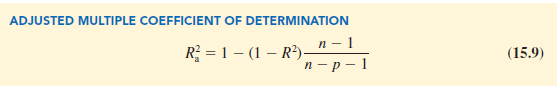
For the Butler Trucking example with n = 10 and p = 2, we have
![]()
Thus, after adjusting for the two independent variables, we have an adjusted multiple coefficient of determination of .8763. This value (expressed as a percentage) is provided in the output in Figure 15.4 as R-Sq(adj) = 87.63%.
Source: Anderson David R., Sweeney Dennis J., Williams Thomas A. (2019), Statistics for Business & Economics, Cengage Learning; 14th edition.
I like this post, enjoyed this one thankyou for posting.
I really like and appreciate your blog.