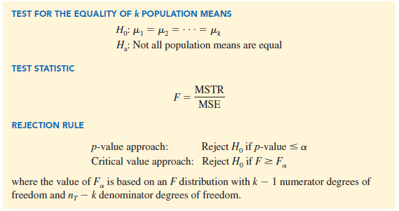
In this section we show how analysis of variance can be used to test for the equality of k population means for a completely randomized design. The general form of the hypotheses tested is

We assume that a simple random sample of size Hj has been selected from each of the k populations or treatments. For the resulting sample data, let

The formulas for the sample mean and sample variance for treatment j are as follows:

The overall sample mean, denoted x, is the sum of all the observations divided by the total number of observations. That is,

If the size of each sample is n, nT = kn; in this case equation (13.3) reduces to

In other words, whenever the sample sizes are the same, the overall sample mean is just the average of the k sample means.
Because each sample in the Chemitech experiment consists of n = 5 observations, the overall sample mean can be computed by using equation (13.5). For the data in Table 13.1 we obtained the following result:

If the null hypothesis is true (μ1 = μ2 = μ3 = μ), the overall sample mean of 60 is the best estimate of the population mean μ.
1. Between-Treatments Estimate of Population Variance
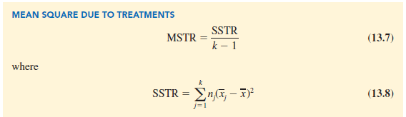
In the preceding section, we introduced the concept of a between-treatments estimate of σ2 and showed how to compute it when the sample sizes were equal. This estimate of σ2 is called the mean square due to treatments and is denoted MSTR. The general formula for computing MSTR is

The numerator in equation (13.6) is called the sum of squares due to treatments and is denoted SSTR. The denominator, k – 1, represents the degrees of freedom associated with SSTR. Hence, the mean square due to treatments can be computed using the following formula.
If H0 is true, MSTR provides an unbiased estimate of σ2. However, if the means of the k populations are not equal, MSTR is not an unbiased estimate of σ2; in fact, in that case, MSTR should overestimate σ2.
For the Chemitech data in Table 13.1, we obtain the following results:
2. Within-Treatments Estimate of Population Variance
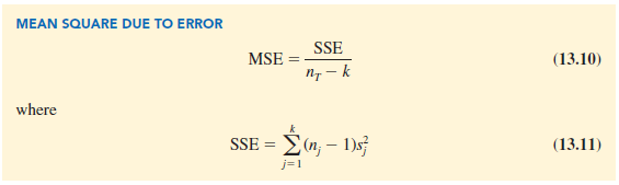
Earlier, we introduced the concept of a within-treatments estimate of s2 and showed how to compute it when the sample sizes were equal. This estimate of s2 is called the mean square due to error and is denoted MSE. The general formula for computing MSE is
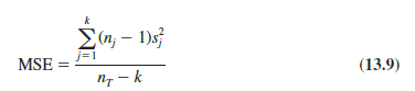
The numerator in equation (13.9) is called the sum of squares due to error and is denoted SSE. The denominator of MSE is referred to as the degrees of freedom associated with SSE. Hence, the formula for MSE can also be stated as follows:
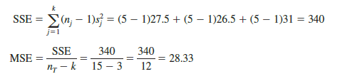
Note that MSE is based on the variation within each of the treatments; it is not influenced by whether the null hypothesis is true. Thus, MSE always provides an unbiased estimate of s2. For the Chemitech data in Table 13.1 we obtain the following results.
3. Comparing the Variance Estimates: The F Test
If the null hypothesis is true, MSTR and MSE provide two independent, unbiased estimates of σ2. Based on the material covered in Chapter 11 we know that for normal populations, the sampling distribution of the ratio of two independent estimates of σ2 follows an F distribution. Hence, if the null hypothesis is true and the ANOVA assumptions are valid, the sampling distribution of MSTR/MSE is an F distribution with numerator degrees of freedom equal to k – 1 and denominator degrees of freedom equal to nT – k. In other words, if the null hypothesis is true, the value of MSTR/MSE should appear to have been selected from this F distribution.
However, if the null hypothesis is false, the value of MSTR/MSE will be inflated because MSTR overestimates a2. Hence, we will reject H0 if the resulting value of MSTR/ MSE appears to be too large to have been selected from an F distribution with k – 1 numerator degrees of freedom and nT – k denominator degrees of freedom. Because the decision to reject H0 is based on the value of MSTR/MSE, the test statistic used to test for the equality of k population means is as follows:

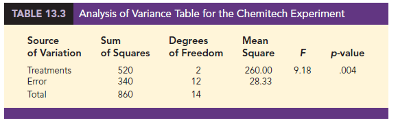
Let us return to the Chemitech experiment and use a level of significance a = .05 to conduct the hypothesis test. The value of the test statistic is

The numerator degrees of freedom is k – 1 = 3 – 1 = 2 and the denominator degrees of freedom is nT – k = 15 – 3 = 12. Because we will only reject the null hypothesis for large values of the test statistic, the p-value is the upper tail area of the F distribution to the right of the test statistic F = 9.18. Figure 13.4 shows the sampling distribution of F = MSTR/MSE, the value of the test statistic, and the upper tail area that is the p-value for the hypothesis test.
From Table 4 of Appendix B we find the following areas in the upper tail of an F distribution with 2 numerator degrees of freedom and 12 denominator degrees of freedom.

Because F = 9.18 is greater than 6.93, the area in the upper tail at F = 9.18 is less than .01. Thus, the p-value is less than .01. Statistical software can be used to show that the exact p-value is .004. With p-value < a = .05, H0 is rejected. The test provides sufficient evidence to conclude that the means of the three populations are not equal. In other words, analysis of variance supports the conclusion that the population mean number of units produced per week for the three assembly methods are not equal.
As with other hypothesis testing procedures, the critical value approach may also be used. With a = .05, the critical F value occurs with an area of .05 in the upper tail of an F distribution with 2 and 12 degrees of freedom. From the F distribution table, we find F.05 = 3.89. Hence, the appropriate upper tail rejection rule for the Chemitech experiment is

With F = 9.18, we reject H0 and conclude that the means of the three populations are not equal. A summary of the overall procedure for testing for the equality of k population means follows.
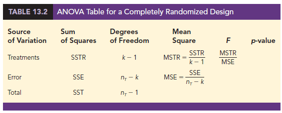
4. ANOVA Table
The results of the preceding calculations can be displayed conveniently in a table referred to as the analysis of variance or ANOVA table. The general form of the ANOVA table for a completely randomized design is shown in Table 13.2; Table 13.3 is the corresponding ANOVA table for the Chemitech experiment. The sum of squares associated with the source of variation referred to as “Total” is called the total sum of squares (SST). Note that the results for the Chemitech experiment suggest that SST = SSTR + SSE, and that the degrees of freedom associated with this total sum of squares is the sum of the degrees of freedom associated with the sum of squares due to treatments and the sum of squares due to error.
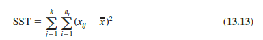
We point out that SST divided by its degrees of freedom nT – 1 is nothing more than the overall sample variance that would be obtained if we treated the entire set of 15 observations as one data set. With the entire data set as one sample, the formula for computing the total sum of squares, SST, is
It can be shown that the results we observed for the analysis of variance table for the Chemitech experiment also apply to other problems. That is,
SST = SSTR + SSE (13.14)
In other words, SST can be partitioned into two sums of squares: the sum of squares due to treatments and the sum of squares due to error. Note also that the degrees of freedom corresponding to SST, nT – 1, can be partitioned into the degrees of freedom corresponding to SSTR, k – 1, and the degrees of freedom corresponding to SSE, nT – k.
The analysis of variance can be viewed as the process of partitioning the total sum of squares and the degrees of freedom into their corresponding sources: treatments and error. Dividing the sum of squares by the appropriate degrees of freedom provides the variance estimates, the F value, and the p-value used to test the hypothesis of equal population means.
5. Computer Results for Analysis of Variance
Using statistical software, analysis of variance computations with large sample sizes or a large number of populations can be performed easily. Appendixes 13.1 and 13.2 show the steps required to use JMP and Excel to perform the analysis of variance computations. In Figure 13.5 we show statistical software output for the Chemitech experiment. The first part of the output contains the familiar ANOVA table format. Comparing Figure 13.5 with Table 13.3, we see that the same information is available, although some of the headings are slightly different. The heading Source is used for the source of variation column, Factor identifies the treatments row, and the sum of squares and degrees of freedom columns are interchanged.
Following the ANOVA table in Figure 13.5, the output contains the respective sample sizes, the sample means, and the standard deviations. In addition, 95% confidence interval estimates of each population mean are given. In developing these confidence interval estimates, MSE is used as the estimate of s2. Thus, the square root of MSE provides the best estimate of the population standard deviation s. This estimate of s in Figure 13.5 is Pooled StDev; it is equal to 5.323. To provide an illustration of how these interval estimates are developed, we will compute a 95% confidence interval estimate of the population mean for Method A.

From our study of interval estimation in Chapter 8, we know that the general form of an interval estimate of a population mean is
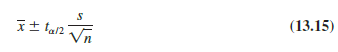
where 5 is the estimate of the population standard deviation s. Because the best estimate of s is provided by the Pooled StDev, we use a value of 5.323 for 5 in expression (13.15). The degrees of freedom for the t value is 12, the degrees of freedom associated with the error sum of squares. Hence, with t.025 = 2.179 we obtain
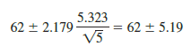
Thus, the individual 95% confidence interval for Method A goes from 62 – 5.19 = 56.81 to 62 + 5.19 = 67.19. Because the sample sizes are equal for the Chemitech experiment, the individual confidence intervals for Method B and Method C are also constructed by adding and subtracting 5.19 from each sample mean.
6. Testing for the Equality of k Population Means:
An Observational Study
We have shown how analysis of variance can be used to test for the equality of k population means for a completely randomized experimental design. It is important to understand that ANOVA can also be used to test for the equality of three or more population means using data obtained from an observational study. As an example, let us consider the situation at National Computer Products, Inc. (NCP).
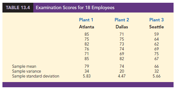
NCP manufactures printers and fax machines at plants located in Atlanta, Dallas, and Seattle. To measure how much employees at these plants know about quality management, a random sample of 6 employees was selected from each plant and the employees selected were given a quality awareness examination. The examination scores for these 18 employees are shown in Table 13.4. The sample means, sample variances, and sample standard deviations for each group are also provided. Managers want to use these data to test the hypothesis that the mean examination score is the same for all three plants.
We define population 1 as all employees at the Atlanta plant, population 2 as all employees at the Dallas plant, and population 3 as all employees at the Seattle plant. Let
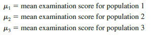
Although we will never know the actual values of m1, m2, and m3, we want to use the sample results to test the following hypotheses:
Note that the hypothesis test for the NCP observational study is exactly the same as the hypothesis test for the Chemitech experiment. Indeed, the same analysis of variance methodology we used to analyze the Chemitech experiment can also be used to analyze the data from the NCP observational study.
Even though the same ANOVA methodology is used for the analysis, it is worth noting how the NCP observational statistical study differs from the Chemitech experimental statistical study. The individuals who conducted the NCP study had no control over how the plants were assigned to individual employees. That is, the plants were already in operation and a particular employee worked at one of the three plants. All that NCP could do was to select a random sample of 6 employees from each plant and administer the quality awareness examination. To be classified as an experimental study, NCP would have had to be able to randomly select 18 employees and then assign the plants to each employee in a random fashion.
Source: Anderson David R., Sweeney Dennis J., Williams Thomas A. (2019), Statistics for Business & Economics, Cengage Learning; 14th edition.
30 Aug 2021
31 Aug 2021
30 Aug 2021
30 Aug 2021
30 Aug 2021
31 Aug 2021