Goodness of Fit Test

In this section we use a chi-square test to determine whether a population being sam­pled has a specific probability distribution. We first consider a population with a histor­ical multinomial probability distribution and use a goodness of fit test to determine if new sample data indicate there has been a change in the population distribution com­pared to the historical distribution. We then consider a situation where an assumption is made that a population has a normal probability distribution. In this case, we use a goodness of fit test to determine if sample data indicate that the assumption of a normal probability distribution is or is not appropriate. Both tests are referred to as goodness of fit tests.

1. Multinomial Probability Distribution

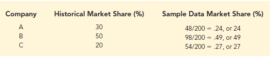
With a multinomial probability distribution, each element of a population is assigned to one and only one of three or more categories. As an example, consider the market share study being conducted by Scott Marketing Research. Over the past year, market shares for a certain product have stabilized at 30% for company A, 50% for company B, and 20% for company C. Since each customer is classified as buying from one of these companies, we have a multinomial probability distribution with three possible outcomes. The probability for each of the three outcomes is as follows.

p_A = probability a customer purchases the company A product

p_B = probability a customer purchases the company B product

p_C = probability a customer purchases the company C product

Using the historical market shares, we have multinomial probability distribution with p_A = .30, p_B = .50, and p_C = .20.

Company C plans to introduce a “new and improved” product to replace its current entry in the market. Company C has retained Scott Marketing Research to determine whether the new product will alter or change the market shares for the three companies. Specifically, the Scott Marketing Research study will introduce a sample of customers to the new company C product and then ask the customers to indicate a preference for the company A product, the company B product, or the new company C product. Based on the sample data, the following hypothesis test can be used to determine if the new company C product is likely to change the historical market shares for the three companies.

The null hypothesis is based on the historical multinomial probability distribution for the market shares. If sample results lead to the rejection of H₀, Scott Marketing Research will have evidence to conclude that the introduction of the new company C product will change the market shares.

Let us assume that the market research firm has used a consumer panel of 200 custom­ers. Each customer was asked to specify a purchase preference among the three alternat­ives: company A’s product, company B’s product, and company C’s new product. The 200 responses are summarized here.

We now can perform a goodness of fit test that will determine whether the sample of 200 customer purchase preferences is consistent with the null hypothesis. Like other chi-square tests, the goodness of fit test is based on a comparison of observed frequencies with the expected frequencies under the assumption that the null hypothesis is true. Hence, the next step is to compute expected purchase preferences for the 200 customers under the assumption that H₀: p_A = .30, p_B = .50, and p_C = .20 is true. Doing so provides the expected frequencies as follows.

Note that the expected frequency for each category is found by multiplying the sample size of 200 by the hypothesized proportion for the category.

The goodness of fit test now focuses on the differences between the observed frequen­cies and the expected frequencies. Whether the differences between the observed and expected frequencies are “large” or “small” is a question answered with the aid of the following chi-square test statistic.

Let us continue with the Scott Marketing Research example and use the sample data to test the hypothesis that the multinomial population has the market share proportions p_A = .30, p_B = .50, and p_C = .20. We will use an a = .05 level of significance. We proceed by using the observed and expected frequencies to compute the value of the test statistic. With the expected frequencies all 5 or more, the computation of the chi-square test statistic is shown in Table 12.9. Thus, we have X² = 7.34.

We will reject the null hypothesis if the differences between the observed and ex­pected frequencies are large. Thus the test of goodness of fit will always be an upper tail test. We can use the upper tail area for the test statistic and the p-value approach to determine whether the null hypothesis can be rejected. With k – 1 = 3 – 1 = 2 degrees of freedom, row two of the chi-square distribution table in Table 12.4 provides the following:

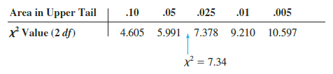
The test statistic X² = 7.34 is between 5.991 and 7.378. Thus, the corresponding upper tail area or p-value must be between .05 and .025. With p-value < .05, we reject H₀ and conclude that the introduction of the new product by company C will alter the historical market shares. JMP or Excel procedures provided in Appendix F can be used to show ^X2 = 7.34 provides a p-value = .0255.

Instead of using the p-value, we could use the critical value approach to draw the same conclusion. With a = .05 and 2 degrees of freedom, the critical value for the test statistic is X²05 = 5.991. The upper tail rejection rule becomes

With 7.34 > 5.991, we reject H₀. The p-value approach and critical value approach provide the same hypothesis testing conclusion.

Now that we have concluded the introduction of a new company C product will alter the market shares for the three companies, we are interested in knowing more about how the market shares are likely to change. Using the historical market shares and the sample data, we summarize the data as follows:

The historical market shares and the sample market shares are compared in the bar chart shown in Figure 12.2. This data visualization process shows that the new product will likely increase the market share for company C. Comparisons for the other two companies indicate that company C’s gain in market share will hurt company A more than company B.

Let us summarize the steps that can be used to conduct a goodness of fit test for a hypothesized multinomial population distribution.

2. Normal Probability distribution

The goodness of fit test for a normal probability distribution is also based on the use of the chi-square distribution. In particular, observed frequencies for several categories of sample data are compared to expected frequencies under the assumption that the population has a normal probability distribution. Because the normal probability distribution is continuous, we must modify the way the categories are defined and how the expected frequencies are computed. Let us demonstrate the goodness of fit test for a normal distribution by consider­ing the job applicant test data for Chemline, Inc., shown in Table 12.10.

Chemline hires approximately 400 new employees annually for its four plants located throughout the United States. The personnel director asks whether a normal distribution applies for the population of test scores. If such a distribution can be used, the distribution would be helpful in evaluating specific test scores; that is, scores in the upper 20%, lower 40%, and so on, could be identified quickly. Hence, we want to test the null hypothesis that the population of test scores has a normal distribution.

Let us first use the data in Table 12.10 to develop estimates of the mean and standard deviation of the normal distribution that will be considered in the null hypothesis. We use the sample mean X and the sample standard deviation 5 as point estimators of the mean and standard deviation of the normal distribution. The calculations follow.

Using these values, we state the following hypotheses about the distribution of the job applicant test scores.

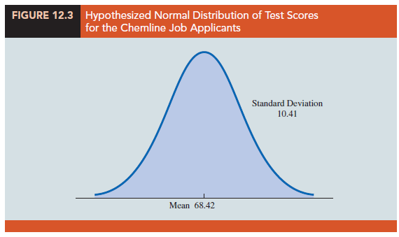
H₀: The population of test scores has a normal distribution with mean 68.42 and standard deviation 10.41

Ha: The population of test scores does not have a normal distribution with mean 68.42 and standard deviation 10.41

The hypothesized normal distribution is shown in Figure 12.3.

With the continuous normal probability distribution, we must use a different procedure for defining the categories. We need to define the categories in terms of intervals of test scores.

Recall the rule of thumb for an expected frequency of at least five in each interval or category. We define the categories of test scores such that the expected frequencies will be at least five for each category. With a sample size of 50, one way of establishing categor­ies is to divide the normal probability distribution into 10 equal-probability intervals (see Figure 12.4). With a sample size of 50, we would expect five outcomes in each inter­val or category, and the rule of thumb for expected frequencies would be satisfied.

Let us look more closely at the procedure for calculating the category boundaries. When the normal probability distribution is assumed, the standard normal probability tables can be used to determine these boundaries. First consider the test score cutting off the lowest 10% of the test scores. From the table for the standard normal distribution we find that the z value for this test score is -1.28. Therefore, the test score of x = 68.42 – 1.28(10.41) = 55.10 provides this cutoff value for the lowest 10% of the scores. For the lowest 20%, we find z = -.84, and thus x = 68.42 – .84(10.41) = 59.68. Working through the normal distribu­tion in that way provides the following test score values.

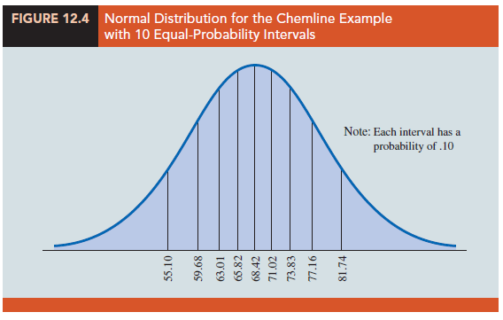
These cutoff or interval boundary points are identified on the graph in Figure 12.4.

With the categories or intervals of test scores now defined and with the known expected frequency of five per category, we can return to the sample data of Table 12.10 and determ­ine the observed frequencies for the categories. Doing so provides the results in Table 12.11.

With the results in Table 12.11, the goodness of fit calculations proceed exactly as be­fore. Namely, we compare the observed and expected results by computing a x² value. The calculations necessary to compute the chi-square test statistic are shown in Table 12.12. We see that the value of the test statistic is x² = 7.2.

To determine whether the computed x² value of 7.2 is large enough to reject H₀, we need to refer to the appropriate chi-square distribution table. Using the rule for computing the number of degrees of freedom for the goodness of fit test, we have k – p – 1 = 10 – 2 – 1 = 7 degrees of freedom based on k = 10 categories and p = 2 parameters (mean and standard deviation) estimated from the sample data.

Suppose that we test the null hypothesis that the distribution for the test scores is a normal distribution with a .10 level of significance. To test this hypothesis, we need to determine the p-value for the test statistic X² = 7.2 by finding the area in the upper tail of a chi-square distribution with 7 degrees of freedom. Using row seven of Table 12.4, we find that X² = 7.2 provides an area in the upper tail greater than .10. Thus, we know that the p-value is greater than .10. JMP or Excel procedures in Appendix F can be used to show X² = 7.2 provides a p-value = .4084. With p-value >.10, the hypothesis that the probability distribution for the Chemline job applicant test scores is a normal probability distribution cannot be rejected. The normal probability distribution may be applied to assist in the interpretation of test scores. A summary of the goodness fit test for a normal probability distribution follows.

Source:  Anderson David R., Sweeney Dennis J., Williams Thomas A. (2019), Statistics for Business & Economics, Cengage Learning; 14th edition.