Inferences About Two Population Variances

In some statistical applications we may want to compare the variances in product quality resulting from two different production processes, the variances in assembly times for two assembly methods, or the variances in temperatures for two heating devices. In making comparisons about the two population variances, we will be using data collected from two independent random samples, one from population 1 and another from population 2. The two sample variances s²₁ and s²₂ will be the basis for making inferences about the two population variances σ²₁ and σ²₂. Whenever the variances of two normal populations are equal (σ²₁   = σ²₂ ) the sampling distribution of the ratio of the two sample variances s²₁ / s²₂  is as follows.

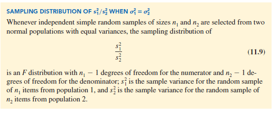
Figure 11.4 is a graph of the F distribution with 20 degrees of freedom for both the numerator and denominator. As indicated by this graph, the F distribution is not symmetric, and the F values can never be negative. The shape of any particular F distribution depends on its numerator and denominator degrees of freedom.

We will use F_a to denote the value of F that provides an area or probability of a in the upper tail of the distribution. For example, as noted in Figure 11.4, F.₀₅ denotes the upper tail area of .05 for an F distribution with 20 degrees of freedom for the numerator and 20 degrees of freedom for the denominator. The specific value of F.₀₅ can be found by referring to the F distribution table, a portion of which is shown in Table 11.3. Using 20 degrees of freedom for the numerator, 20 degrees of freedom for the denominator, and the row corresponding to an area of .05 in the upper tail, we find F.₀₅ = 2.12. Note that the table can be used to find F values for upper tail areas of .10, .05, .025, and .01. See Table 4 of Appendix B for a more extensive table for the F distribution.

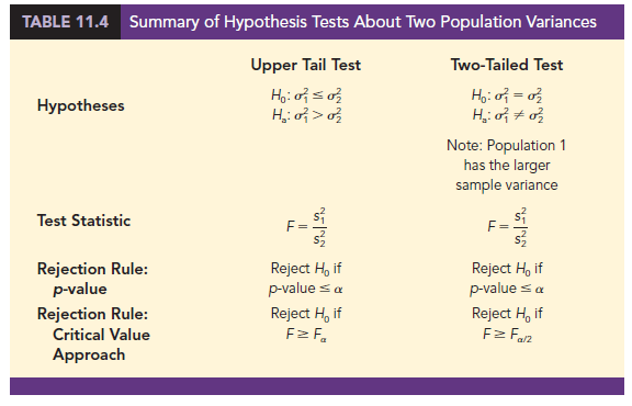
Let us show how the F distribution can be used to conduct a hypothesis test about the variances of two populations. We begin with a test of the equality of two population vari­ances. The hypotheses are stated as follows.

We make the tentative assumption that the population variances are equal. If H₀ is rejected, we will draw the conclusion that the population variances are not equal.

The procedure used to conduct the hypothesis test requires two independent random samples, one from each population. The two sample variances are then computed. We refer to the population providing the larger sample variance as population 1. Thus, a sample size of n₁ and a sample variance of 5 1 correspond to population 1, and a sample size of n₂ and a sample variance of 52 correspond to population 2. Based on the assumption that both popu­lations have a normal distribution, the ratio of sample variances provides the following F test statistic.

Because the F test statistic is constructed with the larger sample variance 52 in the numerator, the value of the test statistic will be in the upper tail of the F distribution. Therefore, the F distribution table as shown in Table 11.3 and in Table 4 of Appendix B need only provide upper tail areas or probabilities. If we did not construct the test statistic in this manner, lower tail areas or probabilities would be needed. In this case, additional calculations or more extensive F distribution tables would be required. Let us now consider an example of a hypothesis test about the equality of two population variances.

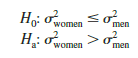
Dullus County Schools is renewing its school bus service contract for the coming year and must select one of two bus companies, the Milbank Company or the Gulf Park Com­pany. We will use the variance of the arrival or pickup/delivery times as a primary meas­ure of the quality of the bus service. Low variance values indicate the more consistent and higher-quality service. If the variances of arrival times associated with the two services are equal, Dullus School administrators will select the company offering the better financial terms. However, if the sample data on bus arrival times for the two companies indicate a significant difference between the variances, the administrators may want to give special consideration to the company with the better or lower variance service. The appropriate hypotheses follow.

If H₀ can be rejected, the conclusion of unequal service quality is appropriate. We will use a level of significance of a = .10 to conduct the hypothesis test.

A sample of 26 arrival times for the Milbank service provides a sample variance of 48 and a sample of 16 arrival times for the Gulf Park service provides a sample vari­ance of 20. Because the Milbank sample provided the larger sample variance, we will denote Milbank as population 1. Using equation (11.10), we find the value of the test statistic:

The corresponding F distribution has n₁ – 1 = 26 – 1 = 25 numerator degrees of freedom and n₂ – 1 = 16 – 1 = 15 denominator degrees of freedom.

As with other hypothesis testing procedures, we can use the p-value approach or the critical value approach to obtain the hypothesis testing conclusion. Table 11.3 shows the following areas in the upper tail and corresponding F values for an F distribution with 25 numerator degrees of freedom and 15 denominator degrees of freedom.

Because F = 2.40 is between 2.28 and 2.69, the area in the upper tail of the distribution is between .05 and .025. For this two-tailed test, we double the upper tail area, which results in a p-value between .10 and .05. Because we selected a = .10 as the level of significance, the p-value < a = .10. Thus, the null hypothesis is rejected. This finding leads to the conclusion that the two bus services differ in terms of pickup/delivery time variances. The recommenda­tion is that the Dullus County School administrators give special consideration to the better or lower variance service offered by the Gulf Park Company.

We can use statistical software to show that the test statistic F = 2.40 provides a two­tailed p-value = .0811. With .0811 < a = .10, the null hypothesis of equal population variances is rejected.

To use the critical value approach to conduct the two-tailed hypothesis test at the a = .10 level of significance, we would select critical values with an area of a/2 = .10/2 = .05 in each tail of the distribution. Because the value of the test statistic computed using equation (11.10) will always be in the upper tail, we only need to determine the upper tail critical value. From Table 11.3, we see that F.₀₅ = 2.28. Thus, even though we use a two­tailed test, the rejection rule is stated as follows.

Because the test statistic F = 2.40 is greater than 2.28, we reject H₀ and conclude that the two bus services differ in terms of pickup/delivery time variances.

One-tailed tests involving two population variances are also possible. In this case, we use the F distribution to determine whether one population variance is significantly greater than the other. A one-tailed hypothesis test about two population variances will always be formulated as an upper tail test:

This form of the hypothesis test always places the p-value and the critical value in the upper tail of the F distribution. As a result, only upper tail F values will be needed, simplifying both the computations and the table for the F distribution.

Let us demonstrate the use of the F distribution to conduct a one-tailed test about the variances of two populations by considering a public opinion survey. Samples of 31 men and 41 women will be used to study attitudes about current political issues. The researcher conducting the study wants to test to see whether the sample data indicate that women show a greater variation in attitude on political issues than men. In the form of the one-tailed hypothesis test given previously, women will be denoted as population 1 and men will be denoted as population 2. The hypothesis test will be stated as follows.

A rejection of H₀ gives the researcher the statistical support necessary to conclude that women show a greater variation in attitude on political issues.

With the sample variance for women in the numerator and the sample variance for men in the denominator, the F distribution will have n₁ – 1 = 41 – 1 = 40 numerator degrees of freedom and n₂ – 1 = 31 – 1 = 30 denominator degrees of freedom. We will use a level of significance a = .05 to conduct the hypothesis test. The survey results provide a sample variance of s2 = 120 for women and a sample variance of s2 = 80 for men. The test statistic is as follows.

Referring to Table 4 in Appendix B, we find that an F distribution with 40 numerator degrees of freedom and 30 denominator degrees of freedom has F.₁₀ = 1.57. Because the test statistic F = 1.50 is less than 1.57, the area in the upper tail must be greater than .10. Thus, we can conclude that the p-value is greater than .10. Using statistical software pro­vides a p-value = .1256. Because the p-value > a = .05, H₀ cannot be rejected. Hence, the sample results do not support the conclusion that women show greater variation in attitude on political issues than men. Table 11.4 provides a summary of hypothesis tests about two population variances.

Source:  Anderson David R., Sweeney Dennis J., Williams Thomas A. (2019), Statistics for Business & Economics, Cengage Learning; 14th edition.