Application 7: Testing Invariance of a Causal Structure (Full Structural Equation Model) with AMOS

1. Key Concepts

• Importance of cross-validation in SEM
• Approaches to cross-validation in SEM
• Testing invariance for a programmed set of measurement and struc­tural parameters based on the Amos multiple-group automated approach
• Interpreting statistical versus practical evidence of tests for invari­ance based on the Amos multiple-group automated approach

In Chapter 4, I highlighted several problematic aspects of post hoc model fitting in structural equation modeling. One approach to addressing problems associated with post hoc model fitting is to apply some mode of cross-validation analysis; this is the focus of the present chapter. In this chapter, we examine a full structural equation model and test for its equivalence across calibration and validation samples of secondary school teachers. Before walking you through this procedure, however, let’s first review some of the issues related to cross-validation.

2. Cross-Validation in Covariance Structure Modeling

Typically, in applications of covariance structure modeling, the researcher tests a hypothesized model and then, based on various goodness-of- fit criteria, concludes that a statistically better-fitting model could be attained by respecifying the model such that particular parameters previ­ously constrained to zero are freely estimated (Breckler, 1990; MacCallum et al., 1992, 1993; MacCallum, Roznowski, Mar, & Reith, 1994). Possibly as a consequence of considerable criticism of covariance structure mod­eling procedures over the past 20 years or so (e.g., Biddle & Marlin, 1987; Breckler, 1990; Cliff, 1983), most researchers engaged in this respecifica­tion process are now generally familiar with the issues. In particular, they are cognizant of the exploratory nature of these follow-up procedures, as well as the fact that additionally specified parameters in the model must be theoretically substantiated.

The pros and cons of post hoc model fitting have been rigorously debated in the literature. Although some have severely criticized the prac­tice (e.g., Cliff, 1983; Cudeck & Browne, 1983), others have argued that as long as the researcher is fully cognizant of the exploratory nature of his or her analyses, the process can be substantively meaningful because practical as well as statistical significance can be taken into account (Byrne et al., 1989; Tanaka & Huba, 1984). However, Joreskog (1993, p. 298) is very clear in stating that “If the model is rejected by the data, the problem is to determine what is wrong with the model and how the model should be modified to fit the data better.” The purists would argue that once a hypothesized model is rejected, that’s the end of the story. More realistic­ally, however, other researchers in this area of study recognize the obvi­ous impracticality in the termination of all subsequent model analyses. Clearly, in the interest of future research, it behooves the investigator to probe deeper into the question of why the model is malfitting (see Tanaka, 1993). As a consequence of the concerted efforts of statistical experts in covariance structure modeling in addressing this issue, there are now sev­eral different approaches that can be used to increase the soundness of findings derived from these post hoc analyses.

Undoubtedly, post hoc model fitting in the analysis of covariance structures is problematic. With multiple model specifications, there is the risk of capitalization on chance factors because model modification may be driven by characteristics of the particular sample on which the model was tested (e.g., sample size, sample heterogeneity) (MacCallum et al., 1992). As a consequence of this sequential testing procedure, there is increased risk of making either a Type I or Type II error and, at this point in time, there is no direct way to adjust for the probability of such error. Because hypothesized covariance structure models represent only approximations of reality and, thus, are not expected to fit real-world phe­nomena exactly (Cudeck & Browne, 1983; MacCallum et al., 1992), most research applications are likely to require the specification of alternative models in the quest for one that fits the data well (Anderson & Gerbing, 1988; MacCallum, 1986). Indeed, this aspect of covariance structure mod­eling represents a serious limitation and, to date, several alternative strategies for model testing have been proposed (see, e.g., Anderson & Gerbing, 1988; Cudeck & Henly, 1991; MacCallum et al., 1992, 1993,1995).

One approach to addressing problems associated with post hoc model-fitting is to employ a cross-validation strategy whereby the final model derived from the post hoc analyses is tested on a second independ­ent sample (or more) from the same population. Barring the availability of separate data samples, albeit a sufficiently large sample, one may wish to randomly split the data into two (or more) parts, thereby making it pos­sible to cross-validate the findings (see Cudeck & Browne, 1983). As such, Sample A serves as the calibration sample on which the initially hypoth­esized model is tested, as well as any post hoc analyses conducted in the process of attaining a well-fitting model. Once this final model is deter­mined, the validity of its structure can then be tested based on Sample B (the validation sample). In other words, the final best-fitting model for the calibration sample becomes the hypothesized model under test for the validation sample.

There are several ways in which the similarity of model structure can be tested (see, e.g., Anderson & Gerbing, 1988; Browne & Cudeck, 1989; Cudeck & Browne, 1983; MacCallum et al., 1994; Whittaker & Stapleton, 2006). For one example, Cudeck and Browne suggested the computation of a Cross-Validation Index (CVI) which measures the distance between the restricted (i.e., model-imposed) variance-covariance matrix for the calibration sample and the unrestricted variance-covariance matrix for the validation sample. Because the estimated predictive validity of the model is gauged by the smallness of the CVI value, evaluation is facilitated by their comparison based on a series of alternative models. It is important to note, however, that the CVI estimate reflects overall discrepancy between “the actual population covariance matrix, Z, and the estimated population covariance matrix reconstructed from the parameter estimates obtained from fitting the model to the sample” (MacCallum et al., 1994, p. 4). More specifically, this global index of discrepancy represents combined effects arising from the discrepancy of approximation (e.g., nonlinear influences among variables) and the discrepancy of estimation (e.g., representative sample; sample size). (For a more extended discussion of these aspects of discrepancy, see Browne & Cudeck, 1989; Cudeck & Henly, 1991; MacCallum et al., 1994.)

More recently, Whittaker and Stapleton (2006), in a comprehensive Monte Carlo simulation study of eight cross-validation indices, deter­mined that certain conditions played an important part in affecting their performance. Specifically, findings showed that whereas the perform­ance of these indices generally improved with increasing factor loading and sample sizes, it tended to be less optimal in the presence of increas­ing nonnormality. (For details related to these findings, as well as the eight cross-validation indices included in this study, see Whittaker & Stapleton, 2006.)

In the present chapter, we examine another approach to cross-validation. Specifically, we use an invariance-testing strategy to test for the replicability of a full structural equation model across groups. The selected application is straightforward in addressing the question of whether a model that has been respecified in one sample replicates over a second independent sample from the same population (for another approach, see Byrne & Baron, 1994).

3. Testing for Invariance across Calibration/Validation Samples

The example presented in this chapter comes from the same study briefly described in Chapter 6 (Byrne, 1994b), the intent of which was three­fold: (a) to validate a causal structure involving the impact of organiza­tional and personality factors on three facets of burnout for elementary, intermediate, and secondary teachers; (b) to cross-validate this model across a second independent sample within each teaching panel; and (c) to test for the invariance of common structural regression (or causal) paths across teaching panels. In contrast to Chapter 6, however, here we focus on (b) in testing for model replication across calibration and val­idation samples of secondary teachers. (For an in-depth examination of invariance-testing procedures within and between the three teacher groups, see Byrne, 1994b.)

It is perhaps important to note that although the present example of cross-validation is based on a full structural equation model, the practice is in no way limited to such applications. Indeed, cross-validation is equally as important for CFA models, and examples of such applications can be found across a variety of disciplines; for those relevant to psychology, see Byrne (1993, 1994a), Byrne and Baron (1994), Byrne and Campbell (1999, Byrne et al., (1993, 1994, 1995, 2004), Byrne, Baron, Larsson, and Melin, 1996), Byrne, Baron, and Balev (1996, 1998); to education, see Benson and Bandalos (1992) and Pomplun and Omar (2003); and to medicine, see Francis, Fletcher, and Rourke (1988), as well as Wang, Wang, and Hoadley (2007). We turn now to the model under study.

The original study from which the present example is taken, comprised a sample of 1,431 high school teachers. For purposes of cross-validation, this sample was randomly split into two; Sample A (n = 716) was used as the calibration group, and Sample B (n = 715) as the validation group. Preliminary analyses conducted for the original study determined two outlying cases which were deleted from all subsequent analyses, thereby rendering final sample sizes of 715 (Sample A) and 714 (Sample B).

4. The Hypothesized Model

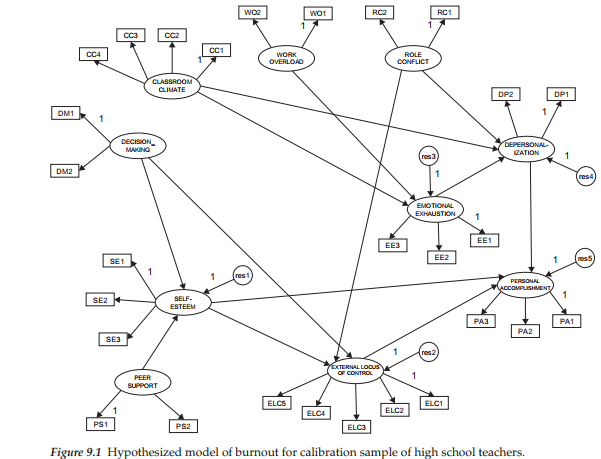
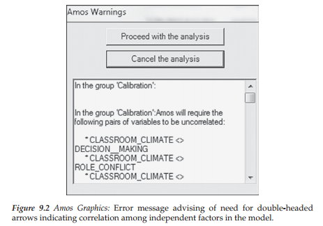
The originally hypothesized model was tested and modified based on data from the calibration sample (Sample A) of high school teachers. The final best-fitting model for this sample is shown schematically in Figure 9.1. It is important to note that, for purposes of clarity, double-headed arrows representing correlations among the independent factors in the model and measurement error terms associated with each of the indicator vari­ables are not included in this figure. Nonetheless, these specifications are essential to the model and must be added before being able to test the model, otherwise Amos will present you with the error message shown in Figure 9.2. Thus, in testing structural equation models using the Amos program, I suggest that you keep two sets of matching model files—one in which you have a cleanly presented figure appropriate for publication purposes, and the other as a working file in which it doesn’t matter how cluttered the figure might be (see, e.g., Figure 9.5).

Establishing a Baseline Model

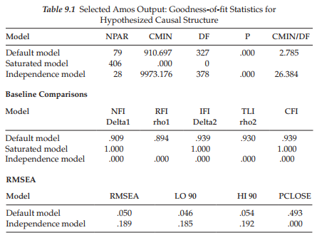
Because analysis of the hypothesized model in the original study was based on the EQS program (Bentler, 2005), for which the modification indices are derived multivariately rather than univariately (as in Amos), I consider it important to test for its validity in establishing a baseline model prior to conducting tests for its invariance across the calibration/validation sam­ples. Initial testing of this model (see Figure 9.1) for the calibration sample yielded the goodness-of-fit statistics reported in Table 9.1. As indicated by a CFI value of .939 (RMSEA = .050), the postulated model of causal structure seems to fit these data well. Nonetheless, a review of both the modifica­tion indices and parameter estimates raises two concerns, which I believe need to be addressed. We turn first to the modification indices reported in Table 9.2, which represent only the structural paths of the model. Here you will quickly notice a large value of 43.899 indicative of an omitted path flowing from Self-esteem (SE) to Emotional Exhaustion (EE). As indicated by the parameter change statistic, addition of this parameter to the model would yield an estimated value of -.568, which is substantial. The negative sign, of course, is substantively appropriate in that low levels of self-esteem are likely to precipitate high levels of emotional exhaustion and vice versa. In light of both the statistical results and the substantive meaningfulness of this structural regression path, I consider that this parameter should be included in the model and the model reestimated.

Before taking a look at the parameter estimates, however, it is import­ant that I make mention of the other large modification index (42.129), representing the same path noted above, albeit in reverse (from Emotional Exhaustion to Self-esteem). Given the similar magnitude (relatively speak­ing) of these two indices, I’m certain that many readers will query why this parameter also is not considered for inclusion in the model. In this regard, I argue against its inclusion in the model for both statistical and substantive reasons. From a statistical perspective, I point to the related parameter change statistic, which shows a negligible value of -.094, clearly indicative of its ineffectiveness as a parameter in the model. From a substantive perspective we need to remember the primary focus of the original study, which was to identify determinants of teacher burnout. Within this framework, specification of a path flowing from Emotional Exhaustion (EE) to Self-esteem (SE) would be inappropriate as the direc­tion of prediction (in this case) runs counter to the intent of the study.

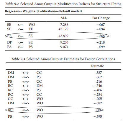
Let’s turn now to Table 9.3 in which estimates of the factor correlations are presented. Circled, you will observe an estimated value of .886 repre­senting the correlation between Role Conflict and Work Overload, thereby indicating an overlap in variance of approximately 78% (.886 x .886). Recall that we noted the same problematic correlation with respect to analyses for elementary teachers (see Chapter 6). As explained in Chapter 6, Role Conflict and Work Overload represent two subscales of the same meas­uring instrument (Teacher Stress Scale). Thus, it seems evident that the related item content is less than optimal in its measurement of behavioral characteristics that distinguish between these two factors.

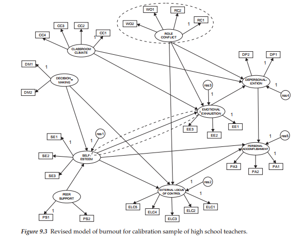
Taking into account the large modification index representing a path from Self-esteem to Emotional Exhaustion, together with the high correlation between the factors of Role Conflict and Work Overload and the same similarity of results for elementary teachers, I consider it appropriate to respecify the hypothesized model such that it includes the new structural path (Self-esteem ^ Emotional Exhaustion) and the deletion of the Work Overload factor, thereby enabling its two indica­tors to load on the Role Conflict factor. This modified model is shown in Figure 9.3.

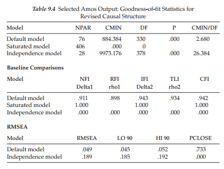
Results from the testing of this respecified model revealed an estimated value of -.719 (S.E. = .093; C.R. = -7.747) for the path from Self-esteem to Emotional Exhaustion, which was somewhat higher than the expected value of -.568. Goodness-of-fit statistics results are reported in Table 9.4. Although the CFI value of .942 (RMSEA = .049) represents only a slight improvement in model fit over the initial CFI value of .039, it nonetheless represents a good fit to the data. Thus, the model shown in Figure 9.3 serves as the baseline model of causal struc­ture that will now be tested for its invariance across calibration and validation samples.

5. Modeling with Amos Graphics

Testing for the Invariance of Causal Structure Using the Automated Multigroup Approach

In Chapter 7, I outlined the general approach to tests for invariance and introduced you to the specification procedures pertinent to both the man­ual and automated approaches related to the Amos program. Whereas the application presented in Chapter 7 focused on the manual approach, the one illustrated in Chapter 8 centered on the automated approach. In this chapter, analyses again are based on the automated procedure, albeit per­tinent to a full causal model.

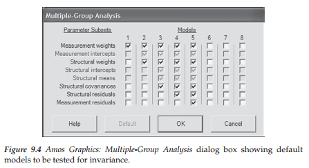
Recall that in Chapter 7, we tested separately for the validity of the multigroup configural model, followed by tests for invariance related sep­arately to each of the measurement and structural models. As noted in Chapter 7 and illustrated in Chapter 8, these tests can be tested simul­taneously using the Amos automated procedure. In the present chapter, we expand on this model-testing process by including both the structural residuals (i.e., error residual variances associated with the dependent fac­tors in the model) and the measurement residuals (i.e., error variances associated with the observed variables). A review of the Multiple-Group Analysis dialog box, shown in Figure 9.4, summarizes the parameters involved in testing for the invariance of these five models. As indicated by the gradual addition of constraints, these models are cumulative in the sense that each is more restrictive than its predecessor.

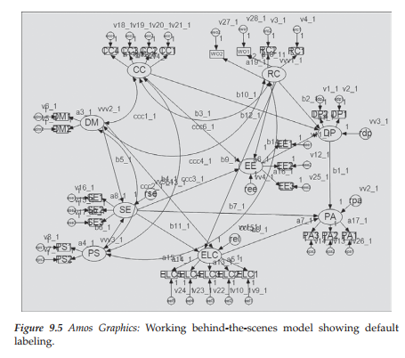
Although I noted in Chapter 7 that inclusion of these structural and measurement residuals in tests for invariance is somewhat rare and commonly considered to be excessively stringent, I include them here for two reasons. First, working with these set of five models provides an excellent vehicle for showing you how the automated approach to invari­ance works, and second, it allows me to reinforce to you the importance of establishing invariance one step at a time (i.e., one set of constrained parameters at a time). Recall my previous notation that, regardless of which model(s) in which a researcher might be interested, Amos auto­matically labels all parameters in the model. For example, although you may wish to activate only the measurement weight model (Model 1), the program will still label all parameters in the model, and not just the fac­tor loadings. Figure 9.5, which represents the behind-the-scenes working multigroup model under test for invariance, provides a good example of this all-inclusive labeling action.

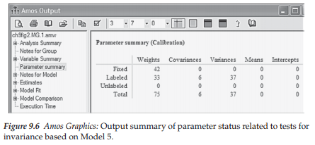
Turning next to Figure 9.6, we find the summary of parameters asso­ciated with the cumulative series of tests for these five models showing the breakdown pertinent to each model tested. In essence, the categoriza­tion of parameters presented in the summary is specific to Model 5. Let’s now dissect this summary in order that you have a clear understanding of what each of these numbers represents and how each was derived; recall that a parameter categorized as “labeled” represents one that is con­strained equal across groups. A breakdown of this parameter summary is as follows:

• Fixed weights (42)—regression paths fixed to a value of 1.0 for 28 measurement error terms, 5 structural residuals, and 9 factor loadings.
• Labeled weights (33)—19 factor loadings and 14 structural paths.
• Labeled covariances (6)—6 factor covariances associated with the 4 (independent) factors.
• Labeled variances (37)—4 (independent) factor variances, 5 residual variances, and 28 error variances.

Selected Amos Output: Goodness-of-fit Statistics for Comparative Tests of Multigroup Invariance

Of primary interest in testing for multigroup invariance are the goodness-of-fit statistics but most importantly, the x², CFI, and RMSEA values as they enable us to determine the extent to which the parameters tested are operating equivalently across the groups. When several tests are conducted simultaneously, Amos computes and reports these results as a set, which makes it easy to compare one model with another. Results for the x² and CFI values related to the series of five models shown in Figure 9.4 are presented in Table 9.5.

Turning to these results, we review first the x² values. The first model in the group represents the configural model for which all parameters are estimated for the calibration and validation groups simultaneously; that is, no parameters are constrained equal across groups. This multigroup model yielded a x² value of 1671.998 with 660 degrees of freedom and serves as the baseline referent against which all subsequent models are compared. In the second model tested (measurement weights), all factor loadings of the indicator variables were constrained equal across groups. Analyses here reveal a x² value of 1703.631 with 679 degrees of freedom. Computation of the Ax² value between this model and the configural model yields a difference of 31.633 with 19 degrees of freedom (because the 19 factor loadings for the validation group were constrained equal to those of the calibration group). This x²-difference value is statistically significant at probability of less than .05. Based on these results, we con­clude that one or more of the factor loadings is not operating equivalently across the two groups. Likewise, Ax² values related to each of the increas­ingly more restrictive models that follow show a steady augmentation of this differential. Overall then, if we use the traditional invariance-testing approach based on the x²-difference test as the basis for determining evi­dence of equivalence, we would conclude that the full structural equation model shown in Figure 9.3 is completely nonequivalent across the calibra­tion and validation groups.

In Table 9.5, I present findings related to the five models checkmarked by default in Amos 23 primarily for the educative purpose of showing

you how this automated process works. Importantly, however, provided with evidence that the factor loadings (see Model 1 in Figure 9.4) are not equivalent across the two groups (Ax²(₁₉) = p < .05), the next step, in practice, is to determine which factor loadings are contributing to these noninvari­ant findings. As such, you then need to conduct these steps in sequence using the labeling technique and procedure illustrated in Chapter 7. The model resulting from this series of tests (the one in which all estimated fac­tor loadings are group-equivalent) then becomes the measurement model used in testing for Model 2. If results from the testing of Model 2 (all struc­tural regression paths constrained equal across groups) are found also to yield evidence of noninvariance, the next task is to identify the paths con­tributing to these findings, and so the same process applied in the case of the factor loadings is once again implemented here for Model 2. Likewise, once a final model is established at this stage (one in which all factor load­ings and structural regression paths are multigroup equivalent), the pro­cess is repeated for each subsequent model to be tested.

Let’s turn now to the alternative approach based on ACFI results. If we were to base our decision-making regarding equivalence of the pos­tulated pattern of causal structure on the more practical approach of the difference in CFI values (see Cheung & Rensvold, 2002; Chapter 7, this volume), we would draw a starkly different conclusion—that, indeed, the model is completely and totally invariant across the two groups. This con­clusion, of course, is based on the fact that the ACFI never exceeded a value of .001. In summary, this conclusion advises that all factor loadings, structural paths, factor covariances, factor residual variances, and meas­urement error variances are operating equivalently across calibration and validation samples.

That researchers seeking evidence of multigroup equivalence related to assessment instruments, theoretical structures, and/or patterns of causal relations can be confronted with such diametrically opposed con­clusions based solely on the statistical approach used in determining this information is extremely disconcerting to say the least. Indeed, it is to be hoped that statisticians engaged in Monte Carlo simulation research related to structural equation modeling will develop more efficient and useful alternative approaches to this decision-making process in the near future. Until such time, however, either we must choose the approach that we believe is most appropriate for the data under study, or we report results related to both.

Source: Byrne Barbara M. (2016), Structural Equation Modeling with Amos: Basic Concepts, Applications, and Programming, Routledge; 3rd edition.