Creating Random Data and Random Samples in Stata

The pseudo-random number function runiform() lies at the heart of Stata’s ability to generate random data or to sample randomly from the data at hand. The Base Reference Manual (Functions) provides a technical description of this 32-bit pseudo-random generator. If we presently have data in memory, then a command such as the following creates a new variable named randnum, having apparently random 16-digit values over the interval [0,1).

. generate randnum = runiform()

We could also create a random dataset from scratch. To do so we first clear other data from memory (if they were valuable, save them first). Next, set the number of observations desired for the new dataset. Explicitly setting the seed number makes it possible to later reproduce the same “random” results. Finally, we generate our random variable. The following commands create a dataset with 10 observations and one variable, called randnum.

In combination with Stata’s algebraic, statistical and special functions, runiform() can simulate values sampled from a variety of theoretical distributions. If we want newvar sampled from a uniform distribution over [0,428) instead of the usual [0,1), we type

. generate newvar = 428 * runiform()

These will still be 16-digit values. Perhaps we want only integers from 1 to 428 (inclusive). The ceiling or ceil() function provides a simple way to do this:

. generate newvar = ceil(428 * runiform())

To simulate 1,000 throws of a six-sided die, type . clear

We theoretically expect 16.67% ones, 16.67% twos and so on, but in any one sample like these 1,000 “throws,” the observed percentages will vary randomly around their expected values.

To simulate 1,000 throws of a pair of six-sided dice, type

We can use _n to begin an artificial dataset as well. The following commands create a new 5,000-observation dataset with one variable named index, containing values from 1 to 5,000.

. set obs 5000
. generate index = _n
. summarize

To generate random variables from a normal (Gaussian) distribution, use the function rnormal(). The following example creates a dataset with 2,000 observations and 2 variables: z from an N(0,1) population, and u from N(500,75).

. clear
. set obs 2000
. generate z = rnormal()
. generate u = rnormal(500,75)

The actual sample means and standard deviations differ slightly from their theoretical values

If z follows a normal distribution, v = e^z follows a lognormal distribution. To form a lognormal variable v based upon a standard normal distribution,

. generate v = exp(rnormal())

Taking logarithms, of course, normalizes a lognormal variable.

To simulate w values drawn randomly from an exponential distribution with mean and standard deviation p = a = 3,

. generate w = -3 * ln(runiform())

For other means and standard deviations, substitute other values for 3. x5 follows a x² (chi-squared) distribution with five degrees of freedom:

. generate x5 = rchi2(5)

y follows a binomial distribution, given 10 trials and success probability .2:

. generate y = rbinomial(10,.2)

t45 follows a Student’s t distribution with 45 degrees of freedom:

. generate t45 = rt(45)

Type help random to see a list of other available functions for generating random variables from beta, gamma, hypergeometric, negative binomial or Poisson distributions.

The drawnorm command provides an alternative way to generate multiple normal variables, and optionally to specify the correlations between them. Using drawnorm to generate 5,000 observations of just one variable from N(0,1), type

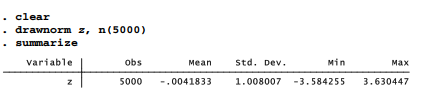
Below, we will create three further variables. Variable x1 is from an N(0,1) population, variable x2 is from N(100,15), and x3 is from N(500,75). Furthermore, we define these variables to have the following population correlations:

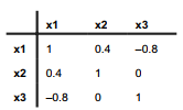
The procedure for creating such data requires first defining the correlation matrix C, and then using C in the drawnorm command:

Compare the sample variables’ correlations and means with the theoretical values given earlier. Random data generated in this fashion can be viewed as samples drawn from theoretical populations. We should not expect the samples to have exactly the theoretical population parameters (in this example, an x3 mean of 500, x1-x2 correlation of 0.4, x1-x3 correlation of -.8, and so forth). Artificial uncorrelated or correlated datasets also can be created via menus and dialog boxes, under

Statistics > Other > Draw a sample from a normal distribution

or

Statistics > Other > Create a dataset with specified correlation structure

The command sample makes unobtrusive use of runiform’s random generator to obtain random samples of the data in memory. For example, to discard all but a 10% random sample of the original data, type

. sample 10

When we add an in or if qualifier, sample applies only to those observations meeting our criteria. For example,

. sample 10 if age < 26

would leave us with a 10% sample of those observations with age less than 26, plus 100% of the original observations with age > 26.

We could also select random samples of a particular size. To discard all but 90 randomly- selected observations from the dataset in memory, type

. sample 90, count

The section in Chapter 14 on Monte Carlo simulations provides further examples of random variable generation.

Source: Hamilton Lawrence C. (2012), Statistics with STATA: Version 12, Cengage Learning; 8th edition.