Test of Independence

An important application of a chi-square test involves using sample data to test for the independence of two categorical variables. For this test we take one sample from a pop­ulation and record the observations for two categorical variables. We will summarize the data by counting the number of responses for each combination of a category for variable 1 and a category for variable 2. The null hypothesis for this test is that the two categorical variables are independent. Thus, the test is referred to as a test of independence. We will illustrate this test with the following example.

A beer industry association conducts a survey to determine the preferences of beer drink­ers for light, regular, and dark beers. A sample of 200 beer drinkers is taken with each person in the sample asked to indicate a preference for one of the three types of beers: light, regular, or dark. At the end of the survey questionnaire, the respondent is asked to provide informa­tion on a variety of demographics including gender: male or female. A research question of interest to the association is whether preference for the three types of beer is independent of the gender of the beer drinker. If the two categorical variables, beer preference and gender, are independent, beer preference does not depend on gender and the preference for light, regular, and dark beer can be expected to be the same for male and female beer drinkers. However, if the test conclusion is that the two categorical variables are not independent, we have evidence that beer preference is associated or dependent upon the gender of the beer drinker. As a result, we can expect beer preferences to differ for male and female beer drink­ers. In this case, a beer manufacturer could use this information to customize its promotions and advertising for the different target markets of male and female beer drinkers.

The hypotheses for this test of independence are as follows:

H₀: Beer preference is independent of gender

H_a: Beer preference is not independent of gender

The sample data will be summarized in a two-way table with beer preferences of light, regular, and dark as one of the variables and gender of male and female as the other variable. Since an objective of the study is to determine if there is difference between the beer preferences for male and female beer drinkers, we consider gender an explanatory variable and follow the usual practice of making the explanatory variable the column variable in the data tabulation table. The beer preference is the categorical response variable and is shown as the row vari­able. The sample results of the 200 beer drinkers in the study are summarized in Table 12.6.

The sample data are summarized based on the combination of beer preference and gender for the individual respondents. For example, 51 individuals in the study were males who preferred light beer, 56 individuals in the study were males who preferred regular beer, and so on. Let us now analyze the data in the table and test for independence of beer preference and gender.

First of all, since we selected a sample of beer drinkers, summarizing the data for each variable separately will provide some insights into the characteristics of the beer drinker population. For the categorical variable gender, we see 132 of the 200 in the sample were male. This gives us the estimate that 132/200 = .66, or 66%, of the beer drinker population is male. Similarly we estimate that 68/200 = .34, or 34%, of the beer drinker population is female.

Thus male beer drinkers appear to outnumber female beer drinkers approximately 2 to 1. Sample proportions or percentages for the three types of beer are

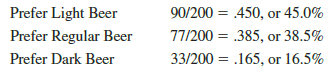
Across all beer drinkers in the sample, light beer is preferred most often and dark beer is preferred least often.

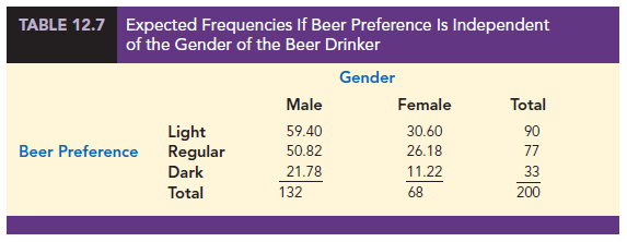
Let us now conduct the chi-square test to determine if beer preference and gender are independent. The computations and formulas used are the same as those used for the chi-square test in Section 12.1. Utilizing the observed frequencies in Table 12.6 for row i and column j, fij, we compute the expected frequencies, eij, under the assumption that the beer preferences and gender are independent. The computation of the expected frequencies follows the same logic and formula used in Section 12.1. Thus the expected frequency for row i and column j is given by

For example, e11 = (90)(132)/200 = 59.40 is the expected frequency for male beer drinkers who would prefer light beer if beer preference is independent of gender. Show that equation (12.4) can be used to find the other expected frequencies shown in Table 12.7.

Following the chi-square test procedure discussed in Section 12.1, we use the following expression to compute the value of the chi-square test statistic.

With r rows and c columns in the table, the chi-square distribution will have (r – 1)(c – 1) degrees of freedom provided the expected frequency is at least 5 for each cell. Thus, in this application we will use a chi-square distribution with (3 – 1)(2 – 1) = 2 degrees of freedom. The complete steps to compute the chi-square test statistic are summarized in Table 12.8.

We can use the upper tail area of the chi-square distribution with 2 degrees of freedom and the p-value approach to determine whether the null hypothesis that beer preference is independent of gender can be rejected. Using row two of the chi-square distribution table shown in Table 12.4, we have the following:

Thus, we see the upper tail area at X² = 6.45 is between .05 and .025, and so the corres­ponding upper tail area or p-value must be between .05 and .025. With p-value < .05, we reject H₀ and conclude that beer preference is not independent of the gender of the beer drinker. Stated another way, the study shows that beer preference can be expected to differ for male and female beer drinkers. JMP or Excel procedures provided in Ap­pendix F can be used to show X² = 6.45 with two degrees of freedom yields a p-value = .0398.

Instead of using the p-value, we could use the critical value approach to draw the same conclusion. With a = .05 and 2 degrees of freedom, the critical value for the chi-square test statistic is X²₀₅ = 5.991. The upper tail rejection region becomes

Reject H₀ if > 5.991

With 6.45 > 5.991, we reject H₀. Again we see that the p-value approach and the critical value approach provide the same conclusion.

While we now have evidence that beer preference and gender are not independent, we will need to gain additional insight from the data to assess the nature of the associ­ation between these two variables. One way to do this is to compute the probability of the beer preference responses for males and females separately. These calculations are as follows:

The bar chart for male and female beer drinkers of the three kinds of beer is shown in Figure 12.1.

What observations can you make about the association between beer preference and gender? For female beer drinkers in the sample, the highest preference is for light beer at 57.35%. For male beer drinkers in the sample, regular beer is most frequently preferred at 42.42%. While female beer drinkers have a higher preference for light beer than males, male beer drinkers have a higher preference for both regular beer and dark beer. Data visu­alization through bar charts such as shown in Figure 12.1 is helpful in gaining insight as to how two categorical variables are associated.

Before we leave this discussion, we summarize the steps for a test of independence.

Finally, if the null hypothesis of independence is rejected, summarizing the probabilities as shown in the above example will help the analyst determine where the association or dependence exists for the two categorical variables.

Source:  Anderson David R., Sweeney Dennis J., Williams Thomas A. (2019), Statistics for Business & Economics, Cengage Learning; 14th edition.