In this section we consider a discrete random variable that is often useful in estimating the number of occurrences over a specified interval of time or space. For example, the random variable of interest might be the number of arrivals at a car wash in one hour, the number of repairs needed in 10 miles of highway, or the number of leaks in 100 miles of pipeline. If the following two properties are satisfied, the number of occurrences is a random variable described by the Poisson probability distribution.
PROPERTIES OF A POISSON EXPERIMENT
-
- The probability of an occurrence is the same for any two intervals of equal length.
- The occurrence or nonoccurrence in any interval is independent of the occurrence or nonoccurrence in any other interval.
The Poisson probability function is defined by equation (5.15).

For the Poisson probability distribution, x is a discrete random variable indicating the number of occurrences in the interval. Since there is no stated upper limit for the number of occurrences, the probability function f (x) is applicable for values x = 0, 1, 2 . . . without limit. In practical applications, x will eventually become large enough so that f(x) is approximately zero and the probability of any larger values of x becomes negligible.
1. An Example Involving Time Intervals
Suppose that we are interested in the number of patients who arrive at the emergency room of a large hospital during a 15-minute period on weekday mornings. If we can assume that the probability of a patient arriving is the same for any two time periods of equal length and that the arrival or nonarrival of a patient in any time period is independent of the arrival or nonarrival in any other time period, the Poisson probability function is applicable. Suppose these assumptions are satisfied and an analysis of historical data shows that the average number of patients arriving in a 15-minute period of time is 10; in this case, the following probability function applies.
![]()
The random variable here is x = number of patients arriving in any 15-minute period.
If management wanted to know the probability of exactly five arrivals in 15 minutes, we would set x = 5 and thus obtain
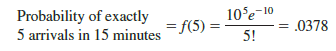
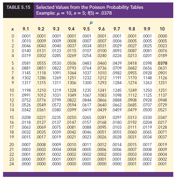
Although this probability was determined by evaluating the probability function with m = 10 and x = 5, it is often easier to refer to a table for the Poisson distribution. The table provides probabilities for specific values of x and m. We included such a table as Table 7 of Appendix B. For convenience, we reproduced a portion of this table as Table 5.15. Note that to use the table of Poisson probabilities, we need know only the values of x and m- From Table 5-15 we see that the probability of five arrivals in a 15-minute period is found by locating the value in the row of the table corresponding to x = 5 and the column of the table corresponding to m = 10- Hence, we obtain f(5) = -0378
In the preceding example, the mean of the Poisson distribution is m = 10 arrivals per 15 minute period- A property of the Poisson distribution is that the mean of the distribution and the variance of the distribution are Thus, the variance for the number of arrivals during 15-minute periods is o2 = 10- The standard deviation is σ = √10 = 3-16. Our illustration involves a 15-minute period, but other time periods can be used- Suppose we want to compute the probability of one arrival in a 3-minute period- Because 10 is the expected number of arrivals in a 15-minute period, we see that 10/15 = 2/3 is the expected number of arrivals in a 1-minute period and that (2/3)(3 minutes) = 2 is the expected number of arrivals in a 3-minute period- Thus, the probability of x arrivals in a 3-minute time period with m = 2 is given by the following Poisson probability function:

The probability of one arrival in a 3-minute period is calculated as follows:

One might expect that because (5 arrivals)/5 = 1 arrival and (15 minutes)/5 = 3 minutes, we would get the same probability for one arrival during a 3-minute period as we do for five arrivals during a 15-minute period- Earlier we computed the probability of five arrivals in a 15-minute period to be -0378- However, note that the probability of one arrival in a three-minute period (-2707) is not the same- When computing a Poisson probability for a different time interval, we must first convert the mean arrival rate to the time period of interest and then compute the probability-
2. An Example Involving Length or Distance Intervals
Let us illustrate an application not involving time intervals in which the Poisson distribution is useful- Suppose we are concerned with the occurrence of major defects in a highway one month after resurfacing- We will assume that the probability of a defect is the same for any two highway intervals of equal length and that the occurrence or nonoccurrence of a defect in any one interval is independent of the occurrence or nonoccurrence of a defect in any other interval- Hence, the Poisson distribution can be applied-
Suppose we learn that major defects one month after resurfacing occur at the average rate of two per mile- Let us find the probability of no major defects in a particular three- mile section of the highway- Because we are interested in an interval with a length of three miles, m = (2 defects/mile)(3 miles) = 6 represents the expected number of major defects over the three-mile section of highway- Using equation (5-15), the probability of no major defects is f(0) = 6°e-6/0! = -0025- Thus, it is unlikely that no major defects will occur in the three-mile section- In fact, this example indicates a 1 – -0025 = -9975 probability of at least one major defect in the three-mile highway section-
Source: Anderson David R., Sweeney Dennis J., Williams Thomas A. (2019), Statistics for Business & Economics, Cengage Learning; 14th edition.
30 Aug 2021
31 Aug 2021
31 Aug 2021
30 Aug 2021
31 Aug 2021
28 Aug 2021