Forecast Accuracy with Time Series Analysis

In this section we begin by developing forecasts for the gasoline time series shown in Table 17.1 using the simplest of all the forecasting methods: an approach that uses the most recent week’s sales volume as the forecast for the next week. For instance, the dis­tributor sold 17 thousand gallons of gasoline in week 1; this value is used as the forecast for week 2. Next, we use 21, the actual value of sales in week 2, as the forecast for week 3, and so on. The forecasts obtained for the historical data using this method are shown in Table 17.7 in the column labeled Forecast. Because of its simplicity, this method is often referred to as a naive forecasting method.

How accurate are the forecasts obtained using this naive forecasting method? To answer this question, we will introduce several measures of forecast accuracy. These measures are used to determine how well a particular forecasting method is able to reproduce the time series data that are already available. By selecting the method that has the best accuracy for the data already known, we hope to increase the likelihood that we will obtain better forecasts for future time periods.

The key concept associated with measuring forecast accuracy is forecast error, defined as

Forecast Error = Ac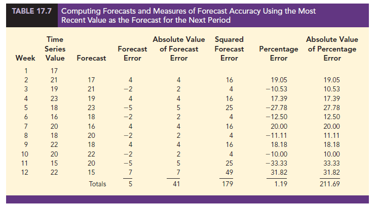tualValue – Forecast

For instance, because the distributor actually sold 21 thousand gallons of gasoline in week 2 and the forecast, using the sales volume in week 1, was 17 thousand gallons, the forecast error in week 2 is

Forecast Error in week 2 = 21 — 17 = 4

The fact that the forecast error is positive indicates that in week 2 the forecasting method underestimated the actual value of sales. Next, we use 21, the actual value of sales in week 2, as the forecast for week 3. Since the actual value of sales in week 3 is 19, the fore­cast error for week 3 is 19 – 21 = -2. In this case, the negative forecast error indicates that in week 3 the forecast overestimated the actual value. Thus, the forecast error may be positive or negative, depending on whether the forecast is too low or too high. A complete summary of the forecast errors for this naive forecasting method is shown in Table 17.7 in the column labeled Forecast Error.

A simple measure of forecast accuracy is the mean or average of the forecast errors. Table 17.7 shows that the sum of the forecast errors for the gasoline sales time series is 5; thus, the mean or average forecast error is 5/11 = .45. Note that although the gasoline time series consists of 12 values, to compute the mean error we divided the sum of the forecast errors by 11 because there are only 11 forecast errors. Because the mean forecast error is positive, the method is underforecasting; in other words, the observed values tend to be greater than the forecasted values. Because positive and negative forecast errors tend to offset one another, the mean error is likely to be small; thus, the mean error is not a very useful measure of forecast accuracy.

The mean absolute error, denoted MAE, is a measure of forecast accuracy that avoids the problem of positive and negative forecast errors offsetting one another.

As you might expect given its name, MAE is the average of the absolute values of the forecast errors. Table 17.7 shows that the sum of the absolute values of the forecast errors is 41; thus,

Another measure that avoids the problem of positive and negative forecast errors offsetting each other is obtained by computing the average of the squared forecast errors. This measure of forecast accuracy, referred to as the mean squared error, is denoted MSE. From Table 17.7, the sum of the squared errors is 179; hence,

The size of MAE and MSE depends upon the scale of the data. As a result, it is dif­ficult to make comparisons for different time intervals, such as comparing a method of forecasting monthly gasoline sales to a method of forecasting weekly sales, or to make comparisons across different time series. To make comparisons like these we need to work with relative or percentage error measures. The mean absolute percentage error, denoted MAPE, is such a measure. To compute MAPE, we must first compute the percentage error for each forecast. For example, the percentage error corresponding to the forecast of 17 in week 2 is computed by dividing the forecast error in week 2 by the actual value in week 2 and multiplying the result by 100. For week 2 the percentage error is computed as follows:

Thus, the forecast error for week 2 is 19.05% of the observed value in week 2. A complete summary of the percentage errors is shown in Table 17.7 in the column labeled Percentage Error. In the next column, we show the absolute value of the percentage error.

Table 17.7 shows that the sum of the absolute values of the percentage errors is 211.69; thus,

Summarizing, using the naive (most recent observation) forecasting method, we obtained the following measures of forecast accuracy:

MAE = 3.73
MSE = 16.27
MAPE = 19.24%

These measures of forecast accuracy simply measure how well the forecasting method is able to forecast historical values of the time series. Now, suppose we want to forecast sales for a future time period, such as week 13. In this case the forecast for week 13 is 22, the actual value of the time series in week 12. Is this an accurate estimate of sales for week 13? Unfortunately, there is no way to address the issue of accuracy associated with forecasts for future time periods. But, if we select a forecasting method that works well for the historical data, and we think that the historical pattern will continue into the future, we should obtain results that will ultimately be shown to be good.

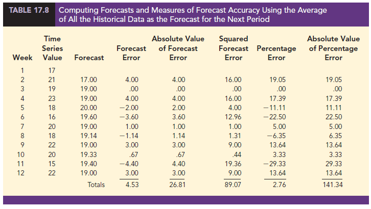
Before closing this section, let’s consider another method for forecasting the gasoline sales time series in Table 17.1. Suppose we use the average of all the historical data available as the forecast for the next period. We begin by developing a forecast for week 2. Since there is only one historical value available prior to week 2, the forecast for week 2 is just the time series value in week 1; thus, the forecast for week 2 is 17 thousand gallons of gasoline. To compute the forecast for week 3, we take the average of the sales values in weeks 1 and 2. Thus,

Similarly, the forecast for week 4 is

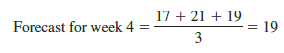
The forecasts obtained using this method for the gasoline time series are shown in Table 17.8 in the column labeled Forecast. Using the results shown in Table 17.8, we obtained the following values of MAE, MSE, and MAPE:

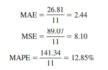
We can now compare the accuracy of the two forecasting methods we have con­sidered in this section by comparing the values of MAE, MSE, and MAPE for each method.

For every measure, the average of past values provides more accurate forecasts than using the most recent observation as the forecast for the next period. In general, if the underlying time series is stationary, the average of all the historical data will always provide the best results.

But suppose that the underlying time series is not stationary. In Section 17.1 we mentioned that changes in business conditions can often result in a time series that has a horizontal pattern shifting to a new level. We discussed a situation in which the gasoline distributor signed a contract with the Vermont State Police to provide gasoline for state police cars located in southern Vermont. Table 17.2 shows the number of gallons of gasoline sold for the original time series and the 10 weeks after signing the new contract, and Figure 17.2 shows the corresponding time series plot. Note the change in level in week 13 for the resulting time series. When a shift to a new level like this occurs, it takes a long time for the forecasting method that uses the average of all the historical data to adjust to the new level of the time series. But, in this case, the simple naive method adjusts very rapidly to the change in level because it uses the most recent observation available as the forecast.

Measures of forecast accuracy are important factors in comparing different forecasting methods, but we have to be careful not to rely upon them too heavily.

Good judgment and knowledge about business conditions that might affect the forecast also have to be carefully considered when selecting a method. And historical forecast accuracy is not the only consideration, especially if the time series is likely to change in the future.

In the next section, we will introduce more sophisticated methods for developing forecasts for a time series that exhibits a horizontal pattern. Using the measures of forecast accuracy developed here, we will be able to determine if such methods provide more accurate forecasts than we obtained using the simple approaches illustrated in this section. The methods that we will introduce also have the advantage of adapting well in situations where the time series changes to a new level. The ability of a forecasting method to adapt quickly to changes in level is an important consideration, especially in short-term forecasting situations.

Source:  Anderson David R., Sweeney Dennis J., Williams Thomas A. (2019), Statistics for Business & Economics, Cengage Learning; 14th edition.