Calculating Portfolio Risk

We have given you an intuitive idea of how diversification reduces risk, but to understand fully the effect of diversification, you need to know how the risk of a portfolio depends on the risk of the individual shares.

Suppose that 60% of your portfolio is invested in Southwest Airlines and the remainder is invested in Amazon. You expect that over the coming year, Amazon will give a return of  10.0% and Southwest 15.0%. The expected return on your portfolio is simply a weighted average of the expected returns on the individual stocks:

Expected portfolio return = (.60 X 15) + (.40 X 10) = 13%

Calculating the expected portfolio return is easy. The hard part is to work out the risk of your portfolio. In the past, the standard deviation of returns was 26.6% for Amazon and 27.9% for Southwest Airlines. You believe that these figures are a good representation of the spread of possible future outcomes. At first you may be inclined to assume that the standard deviation of the portfolio is a weighted average of the standard deviations of the two stocks—that is, (.40 X 26.6) + (.60 X 27.9) = 27.4%. That would be correct only if the prices of the two stocks moved in perfect lockstep. In any other case, diversification reduces the risk below this figure.

The exact procedure for calculating the risk of a two-stock portfolio is given in Figure 7.12. You need to fill in four boxes. To complete the top-left box, you weight the variance of the returns on stock 1(c\) by the square of the proportion invested in it (x²) Similarly, to complete the bottom-right box, you weight the variance of the returns on stock 2(02) by the square of the proportion invested in stock 2(x²).

The entries in these diagonal boxes depend on the variances of stocks 1 and 2; the entries in the other two boxes depend on their covariance. As you might guess, the covariance is a measure of the degree to which the two stocks “covary.” The covariance can be expressed as the product of the correlation coefficient p₁₂ and the two standard deviations:

Covariance between stocks 1 and 2 = ​σ 12  = ​ρ 12 σ 1 σ 2

For the most part stocks tend to move together. In this case the correlation coefficient p₁₂ is positive, and therefore the covariance a₁₂ is also positive. If the prospects of the stocks were wholly unrelated, both the correlation coefficient and the covariance would be zero; and if the stocks tended to move in opposite directions, the correlation coefficient and the covariance would be negative. Just as you weighted the variances by the square of the proportion invested, so you must weight the covariance by the product of the two proportionate holdings x₁ and x₂.

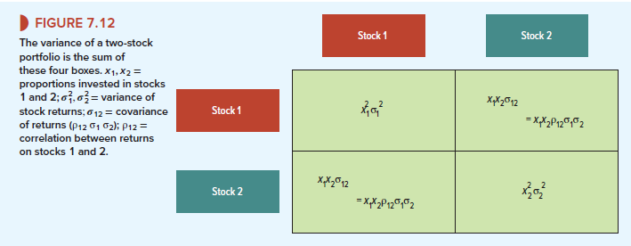
Once you have completed these four boxes, you simply add the entries to obtain the portfolio variance:

The portfolio standard deviation is, of course, the square root of the variance.

Now you can try putting in some figures for Southwest Airlines (LUV) and Amazon (AMZN). We said earlier that if the two stocks were perfectly correlated, the standard devia­tion of the portfolio would lie 40% of the way between the standard deviations of the two stocks. Let us check this out by filling in the boxes with p₁₂ = +1.

The variance of your portfolio is the sum of these entries:

The standard deviation is √749.7 = 27.4% or 60% of the way between 26.6 and 27.9.

Southwest Airlines and Amazon do not move in perfect lockstep. If recent experience is any guide, the correlation between the two stocks is .26. If we go through the same exercise again with p₁₂ = .26, we find

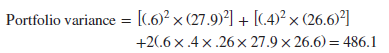
The standard deviation is √486.1 = 22.0%. The risk is now less than 60% of the way between 26.6 and 27.9. In fact, it is almost a fifth less than investing in just one of the two stocks.

The greatest payoff to diversification comes when the two stocks are negatively correlated. Unfortunately, this almost never occurs with real stocks, but just for illustration, let us assume it for Amazon and Southwest Airlines. And as long as we are being unrealistic, we might as well go whole hog and assume perfect negative correlation (p₁₂ = -1). In this case,

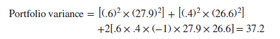
The standard deviation is √37.2 = 6.1%. Risk is almost eliminated. But you can still do better in terms of risk by putting 51.2% of your investment in Amazon and 48.8% in Southwest Airlines. In that case, the standard deviation is almost exactly zero. (Check the calculation yourself.)

When there is perfect negative correlation, there is always a portfolio strategy (represented by a particular set of portfolio weights) that will completely eliminate risk. It’s too bad perfect negative correlation doesn’t really occur between common stocks.

1. General Formula for Computing Portfolio Risk

The method for calculating portfolio risk can easily be extended to portfolios of three or more securities. We just have to fill in a larger number of boxes. Each of those down the diagonal— the red boxes in Figure 7.13—contains the variance weighted by the square of the proportion invested. Each of the other boxes contains the covariance between that pair of securities, weighted by the product of the proportions invested.

EXAMPLE 7.1 ● Limits to Diversification

Did you notice in Figure 7.13 how much more important the covariances become as we add more securities to the portfolio? When there are just two securities, there are equal numbers of variance boxes and of covariance boxes. When there are many securities, the number of covariances is much larger than the number of variances. Thus the variability of a well-diversified portfolio reflects mainly the covariances.

Suppose we are dealing with portfolios in which equal investments are made in each of N stocks. The proportion invested in each stock is, therefore, 1/N. So in each variance box we have (1/N)² times the variance, and in each covariance box we have (1/N)² times the covariance. There are N variance boxes and N² – N covariance boxes. Therefore,

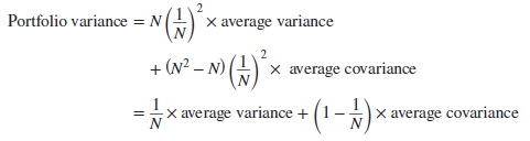
Notice that as N increases, the portfolio variance steadily approaches the average covariance. If the average covariance were zero, it would be possible to eliminate all risk by holding a suf­ficient number of securities. Unfortunately common stocks move together, not independently. Thus most of the stocks that the investor can actually buy are tied together in a web of positive covariances that set the limit to the benefits of diversification. Now we can understand the precise meaning of the market risk portrayed in Figure 7.11. It is the average covariance that constitutes the bedrock of risk remaining after diversification has done its work.

2. Do I Really Have to Add up 36 Million Boxes?

“Adding up the boxes” in Figure 7.13 sounds simple enough, until you remember that there are nearly 6,000 companies listed on the New York and NASDAQ stock exchanges. A port­folio manager who tried to include every one of those companies’ stocks would have to fill up about 6,000 x 6,000 = 36,000,000 boxes! Of course, the boxes above the diagonal line of red boxes in Figure 7.13 match the boxes below. Nevertheless, getting accurate estimates of about 18,000,000 covariances is just impossible. Getting unbiased forecasts of rates of return for about 6,000 stocks is likewise impossible.

Smart investors don’t try. They don’t attempt to forecast portfolio risk or return by “adding up the boxes” for thousands of stocks. But they do understand how portfolio risk is deter­mined by the covariances across securities. (See Example 7.1.) They appreciate the power of diversification, and they want more of it. They want a well-diversified portfolio. Often, they end up holding the entire stock market, as represented by a market index.

You can “buy the market” by purchasing shares in an index fund: a mutual fund or exchange- traded fund (ETF) that invests in the market index that you want to track. Well-run index funds track the market almost exactly and charge very low management fees, often less than 0.1% per year. The most widely used U.S. index is the Standard & Poor’s Composite, which includes 500 of the largest stocks. Index funds have attracted about $5 trillion from investors.

If you have no special information about any of the stocks in the index, it makes sense to be an indexer—that is, to buy the market as a passive rather than active investor. In that case, there is only one box to add up. Just think of the market portfolio as occupying the top-left box in Figure 7.13.

If you want to try out as an active investor, you are well-advised to (1) start with a widely diversified portfolio, for example, a market index fund, and then (2) concentrate on a few stocks as possible additions. You may decide to trade off some investment in the stocks that you are especially fond of against the resulting loss of diversification. In this case, the market index fund occupies the top-left box, and the possible additions occupy a few adjacent boxes.

But our main takeaway so far is this: Smart and serious investors hold widely diversified portfolios; their starting portfolio is often the market itself. How then should such investors assess the risk of individual stocks? Clearly they have to ask how much risk each stock contributes to the risk of a diversified portfolio.

Source:  Brealey Richard A., Myers Stewart C., Allen Franklin (2020), Principles of Corporate Finance, McGraw-Hill Education; 13th edition.