You now have a couple of benchmarks. You know the discount rate for safe projects, and you have an estimate of the rate for average-risk projects. But you don’t know yet how to estimate discount rates for assets that do not fit these simple cases. To do that, you have to learn (1) how to measure risk and (2) the relationship between risks borne and risk premiums demanded.
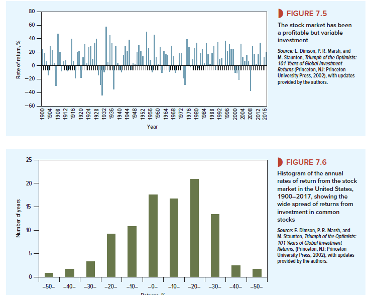
Figure 7.5 shows the 118 annual rates of return for U.S. common stocks. The fluctuations in year-to-year returns are remarkably wide. The highest annual return was 57.6% in 1933—a partial rebound from the stock market crash of 1929-1932. However, there were losses exceeding 25% in six years, the worst being the -43.9% return in 1931.
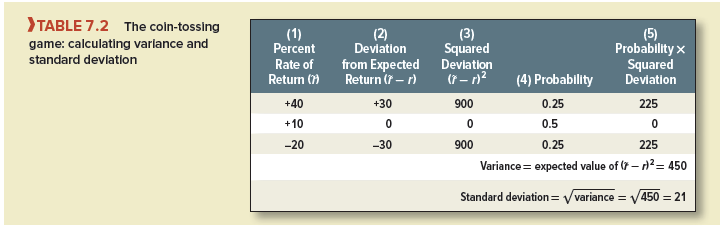
Another way to present these data is by a histogram or frequency distribution. This is done in Figure 7.6, where the variability of year-to-year returns shows up in the wide “spread” of outcomes.
1. Variance and Standard Deviation
The standard statistical measures of spread are variance and standard deviation. The variance of the market return is the expected squared deviation from the expected return. In other words,
![]()
where rm is the actual return and rm is the expected return.15 The standard deviation is simply the square root of the variance:
![]()
Standard deviation is often denoted by σ and variance by σ2.
Here is a very simple example showing how variance and standard deviation are calculated. Suppose that you are offered the chance to play the following game. You start by investing $100. Then two coins are flipped. For each head that comes up, you get back your starting balance plus 20%, and for each tail that comes up, you get back your starting balance less 10%. Clearly there are four equally likely outcomes:
- Head + head: You gain 40%.
- Head + tail: You gain 10%.
- Tail + head: You gain 10%.
- Tail + tail: You lose 20%.
There is a chance of 1 in 4, or .25, that you will make 40%; a chance of 2 in 4, or .5, that you will make 10%; and a chance of 1 in 4, or .25, that you will lose 20%. The game’s expected return is, therefore, a weighted average of the possible outcomes:
Expected return = (.25 X 40) + (.5 X 10) + (.25 X -20) = +10%
Table 7.2 shows that the variance of the percentage returns is 450. Standard deviation is the square root of 450, or 21. This figure is in the same units as the rate of return, so we can say that the game’s variability is 21%.
If outcomes are uncertain, then more things can happen than will happen. The risk of an asset can be completely expressed, as we did for the coin-tossing game, by writing all possible outcomes and the probability of each. In practice, this is cumbersome and often impossible. Therefore, we use variance or standard deviation to summarize the spread of possible outcomes.
These measures are natural indexes of risk.17 If the outcome of the coin-tossing game had been certain, the standard deviation would have been zero. The actual standard deviation is positive because we don’t know what will happen.
Or think of a second game, the same as the first except that each head means a 35% gain and each tail means a 25% loss. Again, there are four equally likely outcomes:
- Head + head: You gain 70%.
- Head + tail: You gain 10%.
- Tail + head: You gain 10%.
- Tail + tail: You lose 50%.
For this game the expected return is 10%, the same as that of the first game. But its standard deviation is double that of the first game, 42% versus 21%. By this measure the second game is twice as risky as the first.
2. Measuring Variability
In principle, you could estimate the variability of any portfolio of stocks or bonds by the procedure just described. You would identify the possible outcomes, assign a probability to each outcome, and grind through the calculations. But where do the probabilities come from? You can’t look them up in the newspaper; newspapers seem to go out of their way to avoid definite statements about prospects for securities. We once saw an article headlined “Bond Prices Possibly Set to Move Sharply Either Way.” Stockbrokers are much the same. Yours may respond to your query about possible market outcomes with a statement like this:
The market currently appears to be undergoing a period of consolidation. For the intermediate term, we would take a constructive view, provided economic recovery continues. The market could be up 20% a year from now, perhaps more if inflation continues low. On the other hand, . . .
The Delphic oracle gave advice, but no probabilities.
Most financial analysts start by observing past variability. Of course, there is no risk in hindsight, but it is reasonable to assume that portfolios with histories of high variability also have the least predictable future performance.
The annual standard deviations and variances observed for our three portfolios over the period 1900-2017 were:
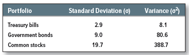
As expected, Treasury bills were the least variable security, and common stocks were the most variable. Government bonds hold the middle ground.
You may find it interesting to compare the coin-tossing game and the stock market as alternative investments. The stock market generated an average annual return of 11.5% with a standard deviation of 19.7%. The game offers 10% and 21%, respectively—slightly lower return and about the same variability. Your gambling friends may have come up with a crude representation of the stock market.
Figure 7.7 compares the standard deviation of stock market returns in 20 countries over the same 118-year period. Portugal occupies high field with a standard deviation of 38.8%, but most of the other countries cluster together with percentage standard deviations in the low 20s.
Of course, there is no reason to suppose that the market’s variability should stay the same over more than a century. For example, Germany, Italy, and Japan now have much more stable economies and markets than they did in the years leading up to and including the Second World War.
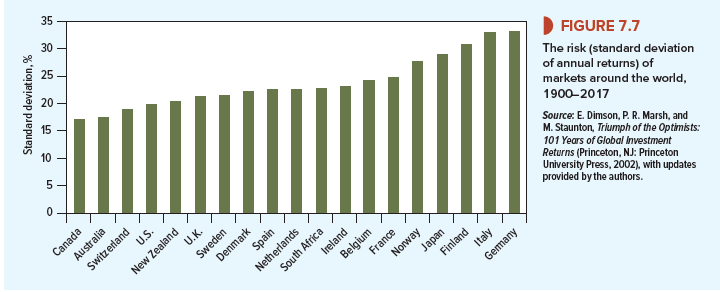
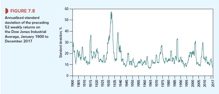
Figure 7.8 does not suggest a long-term upward or downward trend in the volatility of the U.S. stock market.19 Instead there have been periods of both calm and turbulence. In 1995, an unusually tranquil year, the standard deviation of returns was less than 8%. Later, in the financial crisis, the standard deviation spiked at over 40%. By 2017, it had dropped back to its level in 1995.
Market turbulence over shorter daily, weekly, or monthly periods can be amazingly high. On Black Monday, October 19, 1987, the U.S. market fell by 23% on a single day. The market standard deviation for the week surrounding Black Monday was equivalent to 89% per year. Fortunately, volatility reverted to normal levels within a few weeks after the crash.
3. How Diversification Reduces Risk
We can calculate our measures of variability equally well for individual securities and portfolios of securities. Of course, the level of variability over 100 years is less interesting for specific companies than for the market portfolio—it is a rare company that faces the same business risks today as it did a century ago.
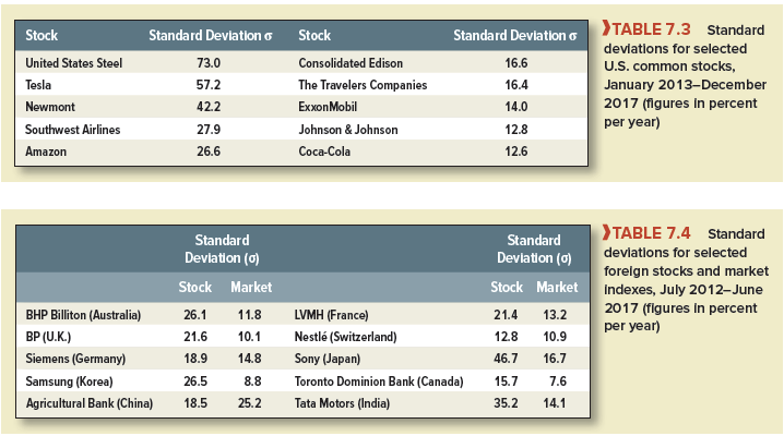
Table 7.3 presents estimated standard deviations for 10 well-known common stocks for a recent five-year period.[4] [5] Do these standard deviations look high to you? They should. The market portfolio’s standard deviation was about 12% during this period. All of our individual stocks had higher volatility. Five of them were more than twice as variable as the market portfolio.
Take a look also at Table 7.4, which shows the standard deviations of some well-known stocks from different countries and of the markets in which they trade. Some of these stocks are more variable than others, but you can see that once again the individual stocks for the most part are more variable than the market indexes.
This raises an important question: The market portfolio is made up of individual stocks, so why doesn’t its variability reflect the average variability of its components? The answer is that diversification reduces variability.
Selling umbrellas is a risky business; you may make a killing when it rains, but you are likely to lose your shirt in a heat wave. Selling ice cream is not safe; you do well in the heat wave, but business is poor in the rain. Suppose, however, that you invest in both an umbrella shop and an ice cream shop. By diversifying your business across two businesses, you make an average level of profit come rain or shine.
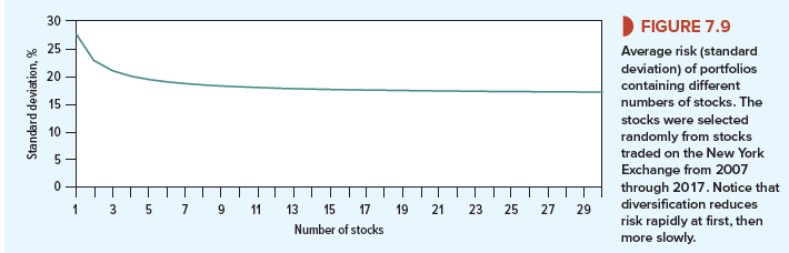
For investors, even a little diversification can provide a substantial reduction in variability. Suppose you calculate and compare the standard deviations between 2007 and 2017 of one- stock portfolios, two-stock portfolios, five-stock portfolios, and so forth. You can see from Figure 7.9 that diversification can cut the variability of returns by about a third. Notice also that you can get most of this benefit with relatively few stocks: The improvement is much smaller when the number of securities is increased beyond, say, 20 or 30.
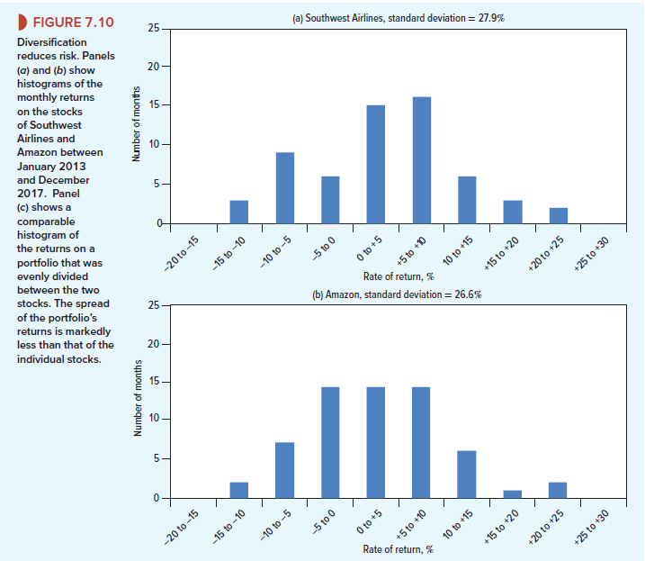
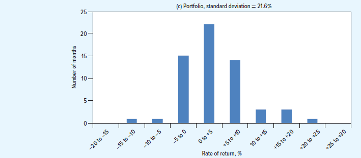
Diversification works because prices of different stocks do not move exactly together. Statisticians make the same point when they say that stock price changes are less than perfectly correlated. Look, for example, at Figure 7.10. Panels (a) and (b) show the spread of monthly returns on the stocks of Southwest Airlines and Amazon. Although the two stocks enjoyed a fairly bumpy ride, they did not move in exact lockstep. Often a decline in the value of one stock was offset by a rise in the price of the other.21 So, if you had split your portfolio evenly between the two stocks, you could have reduced the monthly fluctuations in the value of your investment. You can see this from panel (c), which shows that if your portfolio had been evenly divided between the two stocks, there would have been many more months when the return was just middling and far fewer cases of extreme returns.
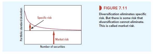
The risk that potentially can be eliminated by diversification is called specific risk.22 Specific risk stems from the fact that many of the perils that surround an individual company are peculiar to that company and perhaps its immediate competitors. But there is also some risk that you can’t avoid, regardless of how much you diversify. This risk is generally known as market risk.23 Market risk stems from the fact that there are other economywide perils that threaten all businesses. That is why stocks have a tendency to move together. And that is why investors are exposed to market uncertainties, no matter how many stocks they hold.
In Figure 7.11, we have divided risk into its two parts—specific risk and market risk. If you have only a single stock, specific risk is very important; but once you have a portfolio of 20 or more stocks, diversification has done the bulk of its work. For a reasonably well-diversified portfolio, only market risk matters. Therefore, the predominant source of uncertainty for a diversified investor is that the market will rise or plummet, carrying the investor’s portfolio with it.
I enjoy your piece of work, thankyou for all the good posts.
Lovely just what I was searching for.Thanks to the author for taking his clock time on this one.