In practical capital budgeting, a single risk-adjusted rate is used to discount all future cash flows. This assumes that project risk does not change over time, but remains constant year- in and year-out. We know that this cannot be strictly true, for the risks that companies are exposed to are constantly shifting. We are venturing here onto somewhat difficult ground, but there is a way to think about risk that can suggest a route through. It involves converting the expected cash flows to certainty equivalents. First we work through an example showing what certainty equivalents are. Then, as a reward for your investment, we use certainty equivalents to uncover what you are really assuming when you discount a series of future cash flows at a single risk-adjusted discount rate. We also value a project where risk changes over time and ordinary discounting fails. Your investment will be rewarded still more when we cover options in Chapters 20 and 21 and forward and futures pricing in Chapter 26. Option-pricing formulas discount certainty equivalents. Forward and futures prices are certainty equivalents.
1. Valuation by Certainty Equivalents
Think back to the simple real estate investment that we used in Chapter 2 to introduce the concept of present value. You are considering construction of an office building that you plan to sell after one year for $800,000. That cash flow is uncertain with the same risk as the market, so p = 1. The risk-free interest rate is rf = 7%, but you discount the $800,000 payoff at a risk- adjusted rate of r = 12%. This gives a present value of 800,000/1.12 = $714,286.
Suppose a real estate company now approaches and offers to fix the price at which it will buy the building from you at the end of the year. This guarantee would remove any uncertainty about the payoff on your investment. So you would accept a lower figure than the uncertain payoff of $800,000. But how much less? If the building has a present value of $714,286 and the interest rate is 7%, then
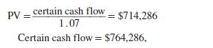
In other words, a certain cash flow of $764,286 has exactly the same present value as an expected but uncertain cash flow of $800,000. The cash flow of $764,286 is therefore known as the certainty-equivalent cash flow. To compensate for both the delayed payoff and the uncertainty in real estate prices, you need a return of 800,000 – 714,286 = $85,714. One part of this difference compensates for the time value of money. The other part ($800,000 – 764,286 = $35,714) is a markdown or haircut to compensate for the risk attached to the forecasted cash flow of $800,000.
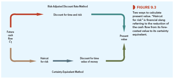
Our example illustrates two ways to value a risky cash flow:
Method 1: Discount the risky cash flow at a risk-adjusted discount rate r that is greater than rf.[1] The risk-adjusted discount rate adjusts for both time and risk. This is illustrated by the clockwise route in Figure 9.3.
Method 2: Find the certainty-equivalent cash flow and discount at the risk-free interest rate rf. When you use this method, you need to ask, What is the smallest certain payoff for which I would exchange the risky cash flow? This is called the certainty equivalent, denoted by CEQ. Since CEQ is the value equivalent of a safe cash flow, it is discounted at the risk-free rate. The certainty-equivalent method makes separate adjustments for risk and time. This is illustrated by the counterclockwise route in Figure 9.3.
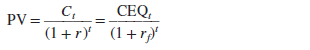
We now have two identical expressions for the PV of a cash flow in period 1:
![]()
For cash flows two, three, or t years away,
2. When to Use a Single Risk-Adjusted Discount Rate for Long-Lived Assets
We are now in a position to examine what is implied when a constant risk-adjusted discount rate is used to calculate a present value.
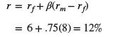
Consider two simple projects. Project A is expected to produce a cash flow of $100 million for each of three years. The risk-free interest rate is 6%, the market risk premium is 8%, and project A’s beta is .75. You therefore calculate A’s opportunity cost of capital as follows:
Discounting at 12% gives the following present value for each cash flow:
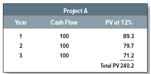
Now compare these figures with the cash flows of project B. Notice that B’s cash flows are lower than A’s; B’s flows are safe, however, and therefore they are discounted at the risk-free interest rate. The present value of each year’s cash flow is identical for the two projects.
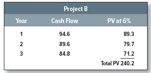
In year 1 project A has a risky cash flow of 100. This has the same PV as the safe cash flow of 94.6 from project B. Therefore, 94.6 is the certainty equivalent of 100. Since the two cash flows have the same PV, investors must be willing to give up 100 – 94.6 = 5.4 in expected year-1 income in order to get rid of the uncertainty.
In year 2, project A has a risky cash flow of 100, and B has a safe cash flow of 89.6. Again both flows have the same PV. Thus, to eliminate the uncertainty in year 2, investors are prepared to give up 100 – 89.6 = 10.4 of future income. To eliminate uncertainty in year 3, they are willing to give up 100 – 84.8 = 15.2 of future income.
To value project A, you discounted each cash flow at the same risk-adjusted discount rate of 12%. Now you can see what is implied when you did that. By using a constant rate, you effectively made a larger deduction for risk from the later cash flows:
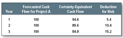
The second cash flow is riskier than the first because it is exposed to two years of market risk. The third cash flow is riskier still because it is exposed to three years of market risk. This increased risk is reflected in the certainty equivalents that decline by a constant proportion each period.[3]
Therefore, use of a constant risk-adjusted discount rate for a stream of cash flows assumes that risk accumulates at a constant rate as you look farther out into the future. That will be the case if the project’s beta remains constant.
3. A Common Mistake
You sometimes hear people say that because distant cash flows are riskier, they should be discounted at a higher rate than earlier cash flows. That is quite wrong: We have just seen that using the same risk-adjusted discount rate for each year’s cash flow implies a larger deduction for risk from the later cash flows. The reason is that the discount rate compensates for the risk borne per period. The more distant the cash flows, the greater the number of periods and the larger the total risk adjustment.
4. When You Cannot Use a Single Risk-Adjusted Discount Rate for Long-Lived Assets
Sometimes you will encounter problems where the use of a single risk-adjusted discount rate will get you into trouble. For example, later in the book, we look at how options are valued. Because an option’s risk is continually changing, the certainty-equivalent method needs to be used.
Here is a disguised, simplified, and somewhat exaggerated version of an actual project proposal that one of the authors was asked to analyze. The scientists at Vegetron have come up with an electric mop, and the firm is ready to go ahead with pilot production and test marketing. The preliminary phase will take one year and cost $125,000. Management feels that there is only a 50% chance that pilot production and market tests will be successful. If they are, then Vegetron will build a $1 million plant that would generate an expected annual cash flow in perpetuity of $250,000 a year after taxes. If they are not successful, the project will have to be dropped.
The expected cash flows (in thousands of dollars) are
C0 = -125
C1 = 50% chance of – 1,000 and 50% chance of 0
= .5(-1,000) + .5(0) = -500
Ct for t = 2, 3, . . . = 50% chance of 250 and 50% chance of 0
= .5(250) + .5(0) = 125
Management has little experience with consumer products and considers this a project of extremely high risk.[4] Therefore management discounts the cash flows at 25%, rather than at Vegetron’s normal 10% standard:
![]()
This seems to show that the project is not worthwhile.
Management’s analysis is open to criticism if the first year’s experiment resolves a high proportion of the risk. If the test phase is a failure, then there is no risk at all—the project is certain to be worthless. If it is a success, there could well be only normal risk from then on. That means there is a 50% chance that in one year Vegetron will have the opportunity to invest in a project of normal risk, for which the normal discount rate of 10% would be appropriate. Thus the firm has a 50% chance to invest $1 million in a project with a net present value of $1.5 million:
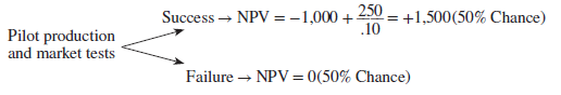
Thus we could view the project as offering an expected payoff of .5(1,500) + .5(0) = 750, or $750,000, at t = 1 on a $125,000 investment at t = 0. Of course, the certainty equivalent of the payoff is less than $750,000, but the difference would have to be very large to justify rejecting the project. For example, if the certainty equivalent is half the forecasted cash flow (an extremely large cash flow haircut) and the risk-free rate is 7%, the project is worth $225,500:
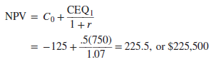
This is not bad for a $125,000 investment—and quite a change from the negative-NPV that management got by discounting all future cash flows at 25%.
Would love to perpetually get updated outstanding blog! .
I enjoy your writing style really loving this internet site.