Suppose that a coal-mining corporation needs to assess the risk of investing in a new company headquarters. The asset beta for coal mining is not helpful. You need to know the beta of real estate. Fortunately, portfolios of commercial real estate are traded. For example, you could estimate asset betas from returns on Real Estate Investment Trusts (REITs) specializing in commercial real estate.[1] The REITs would serve as traded comparables for the proposed office building. You could also turn to indexes of real estate prices and returns derived from sales and appraisals of commercial properties.[2]
A company that wants to set a cost of capital for one particular line of business typically looks for pure plays in that line of business. Pure-play companies are public firms that specialize in one activity. For example, suppose that J&J wants to set a cost of capital for its pharmaceutical business. It could estimate the average asset beta or cost of capital for pharmaceutical companies that have not diversified into consumer products like Band-Aid® bandages or baby powder.
Overall company costs of capital are almost useless for conglomerates. Conglomerates diversify into several unrelated industries, so they have to consider industry-specific costs of capital. They therefore look for pure plays in the relevant industries. Take Richard Branson’s Virgin Group as an example. The group combines many different companies, including airlines (Virgin Atlantic) and train services (Virgin Rail Group). Fortunately, there are many examples of pure-play airlines and train operators. The trick is picking the comparables with business risks that are most similar to Virgin’s companies.
Sometimes good comparables are not available or are not a good match to a particular project. Then the financial manager has to exercise his or her judgment. Here we offer the following advice:
- Think about the determinants of asset betas. Often, the characteristics of high- and low- beta assets can be observed when the beta itself cannot be.
- Don’t be fooled by diversifiable risk.
- Avoid fudge factors. Don’t give in to the temptation to add fudge factors to the discount rate to offset things that could go wrong with the proposed investment. Adjust cashflow forecasts instead.
1. What Determines Asset Betas?
Cyclicality Many people’s intuition associates risk with the variability of earnings or cash flow. But much of this variability reflects diversifiable risk. Lone prospectors searching for gold look forward to extremely uncertain future income, but whether they strike it rich is unlikely to depend on the performance of the market portfolio. Even if they do find gold, they do not bear much market risk. Therefore, an investment in gold prospecting has a high standard deviation but a relatively low beta.
What really counts is the strength of the relationship between the firm’s earnings and the aggregate earnings on all real assets. We can measure this either by the earnings beta or by the cash-flow beta. These are just like a real beta except that changes in earnings or cash flow are used in place of rates of return on securities. Firms with high earnings or cash-flow betas are more likely to have high asset betas.
This means that cyclical firms—firms whose revenues and earnings are strongly dependent on the state of the business cycle—tend to be high-beta firms. Thus, you should demand a higher rate of return from investments whose performance is strongly tied to the performance of the economy. Examples of cyclical businesses include airlines, luxury resorts and restaurants, construction, and steel. (Much of the demand for steel depends on construction and capital investment.) Examples of less-cyclical businesses include food and tobacco products and established consumer brands such as J&J’s baby products. MBA programs are another example because spending a year or two at a business school is an easier choice when jobs are scarce. Applications to top MBA programs increase in recessions.
Operating Leverage A production facility with high fixed costs, relative to variable costs, is said to have high operating leverage. High operating leverage means a high asset beta. Let us see how this works.
The cash flows generated by an asset can be broken down into revenue, fixed costs, and variable costs:
Cash flow = revenue – fixed cost – variable cost
Costs are variable if they depend on the rate of output. Examples are raw materials, sales commissions, and some labor and maintenance costs. Fixed costs are cash outflows that occur regardless of whether the asset is active or idle, for example, property taxes or the wages of workers under contract.
We can break down the asset’s present value in the same way:
PV(asset) = PV(revenue) – PV(fixed cost) – PV(variable cost)
Or equivalently
PV(revenue) = PV(fixed cost) + PV(variable cost) + PV(asset)
Those who receive the fixed costs are like debtholders in the project; they simply get a fixed payment. Those who receive the net cash flows from the asset are like holders of common stock; they get whatever is left after payment of the fixed costs.
We can now figure out how the asset’s beta is related to the betas of the values of revenue and costs. The beta of PV(revenue) is a weighted average of the betas of its component parts:
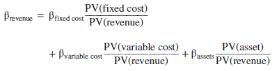
The fixed-cost beta should be close to zero; whoever receives the fixed costs receives a fixed stream of cash flows. The betas of the revenues and variable costs should be approximately the same, because they respond to the same underlying variable, the rate of output. Therefore we can substitute prevenue for pvariable cost and solve for the asset beta. Remember, we are assuming Pfixed cost = 0. Also, PV(revenue) – PV(variable cost) = PV(asset) + PV(fixed cost).
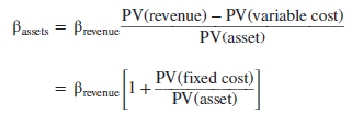
Thus, given the cyclicality of revenues (reflected in Prevenue), the asset beta is proportional to the ratio of the present value of fixed costs to the present value of the project.
Now you have a rule of thumb for judging the relative risks of alternative designs or technologies for producing the same project. Other things being equal, the alternative with the higher ratio of fixed costs to project value will have the higher project beta. Empirical tests confirm that companies with high operating leverage actually do have high betas.[4]
We have interpreted fixed costs as costs of production, but fixed costs can show up in other forms, for example, as future investment outlays. Suppose that an electric utility commits to build a large electricity-generating plant. The plant will take several years to build, and the costs are fixed obligations. Our operating leverage formula still applies, but with PV(future investment) included in PV(fixed costs). The commitment to invest therefore increases the plant’s asset beta. Of course PV(future investment) decreases as the plant is constructed and disappears when the plant is up and running. Therefore the plant’s asset beta is only temporarily high during construction.
Other Sources of Risk So far we have focused on cash flows. Cash-flow risk is not the only risk. A project’s value is equal to the expected cash flows discounted at the risk-adjusted discount rate r. If either the risk-free rate or the market risk premium changes, then r will change and so will the project value. A project with very long-term cash flows is more exposed to such shifts in the discount rate than one with short-term cash flows. This project will, therefore, have a high beta even though it may not have high operating leverage or cyclicality.[5]
You cannot hope to estimate the relative risk of assets with any precision, but good managers examine each project from a variety of angles and look for clues as to its riskiness. They know that high market risk is a characteristic of cyclical ventures, of projects with high fixed costs and of projects that are sensitive to marketwide changes in the discount rate. They think about the major uncertainties affecting the economy and consider how their projects are affected by these uncertainties.
2. Don’t Be Fooled by Diversifiable Risk
In this chapter, we have defined risk as the asset beta for a firm, industry, or project. But in everyday usage, “risk” simply means “bad outcome.” People think of the risks of a project as a list of things that can go wrong. For example,
- A geologist looking for oil worries about the risk of a dry hole.
- A pharmaceutical-company scientist worries about the risk that a new drug will have unacceptable side effects.
- A plant manager worries that new technology for a production line will fail to work, requiring expensive changes and repairs.
- A telecom CFO worries about the risk that a communications satellite will be damaged by space debris. (This was the fate of an Iridium satellite in 2009, when it collided with Russia’s defunct Cosmos 2251. Both were blown to smithereens.)
Notice that these risks are all diversifiable. For example, the Iridium-Cosmos collision was definitely a zero-beta event. These hazards do not affect asset betas and should not affect the discount rate for the projects.
Sometimes, financial managers increase discount rates in an attempt to offset these risks. This makes no sense. Diversifiable risks do not increase the cost of capital.
Example 9.1 • Allowing for Possible Bad Outcomes
Project Z will produce just one cash flow, forecasted at $1 million at year 1. It is regarded as average risk, suitable for discounting at a 10% company cost of capital:
![]()
But now you discover that the company’s engineers are behind schedule in developing the technology required for the project. They are confident it will work, but they admit to a small chance that it will not. You still see the most likely outcome as $1 million, but you also see some chance that project Z will generate zero cash flow next year.
Now the project’s prospects are clouded by your new worry about technology. It must be worth less than the $909,100 you calculated before that worry arose. But how much less? There is some discount rate (10% plus a fudge factor) that will give the right value, but we do not know what that adjusted discount rate is.
We suggest you reconsider your original $1 million forecast for project Z’s cash flow. Project cash flows are supposed to be unbiased forecasts that give due weight to all possible outcomes, favorable and unfavorable. Managers making unbiased forecasts are correct on average. Sometimes, their forecasts will turn out high, other times low, but their errors will average out over many projects.
If you forecast a cash flow of $1 million for projects like Z, you will overestimate the average cash flow, because every now and then you will hit a zero. Those zeros should be “averaged in” to your forecasts.
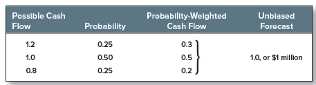
For many projects, the most likely cash flow is also the unbiased forecast. If there are three possible outcomes with the probabilities shown below, the unbiased forecast is $1 million. (The unbiased forecast is the sum of the probability-weighted cash flows.)
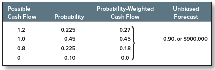
This might describe the initial prospects of project Z. But if technological uncertainty introduces a 10% chance of a zero cash flow, the unbiased forecast could drop to $900,000:
The present value is
![]()
Managers often work out a range of possible outcomes for major projects, sometimes with explicit probabilities attached. We give more elaborate examples and further discussion in Chapter 10. But even when outcomes and probabilities are not explicitly written down, the manager can still consider the good and bad outcomes as well as the most likely one. When the bad outcomes outweigh the good, the cash-flow forecast should be reduced until balance is regained.
Step 1, then, is to do your best to make unbiased forecasts of a project’s cash flows. Unbiased forecasts incorporate all possible outcomes, including those that are specific to your project and those that stem from economywide events. Step 2 is to consider whether diversified investors would regard the project as more or less risky than the average project. In this step only market risks are relevant.
3. Avoid Fudge Factors in Discount Rates
Think back to our example of project Z, where we reduced forecasted cash flows from $1 million to $900,000 to account for a possible failure of technology. The project’s PV was reduced from $909,100 to $818,000. You could have gotten the right answer by adding a fudge factor to the discount rate and discounting the original forecast of $1 million. But you have to think through the possible cash flows to get the fudge factor, and once you forecast the cash flows correctly, you don’t need the fudge factor.
Fudge factors in discount rates are dangerous because they displace clear thinking about future cash flows. Here is an example.
Example 9.2 • Correcting for Optimistic Forecasts
The chief financial officer (CFO) of EZ2 Corp. is disturbed to find that cash-flow forecasts for its investment projects are almost always optimistic. On average they are 10% too high. He therefore decides to compensate by adding 10% to EZ2’s WACC, increasing it from 12% to 22%.18
Suppose the CFO is right about the 10% upward bias in cash-flow forecasts. Can he just add 10% to the discount rate?
Project ZZ has level forecasted cash flows of $1,000 per year lasting for 15 years. The first two lines of Table 9.2 show these forecasts and their PVs discounted at 12%. Lines 3 and 4 show the corrected forecasts, each reduced by 10%, and the corrected PVs, which are (no surprise) also reduced by 10% (line 5). Line 6 shows the PVs when the uncorrected forecasts are discounted at 22%. The final line 7 shows the percentage reduction in PVs at the 22% discount rate, compared to the unadjusted PVs in line 2.
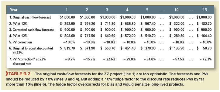
Line 5 shows the correct adjustment for optimism (10%). Line 7 shows what happens when a 10% fudge factor is added to the discount rate. The effect on the first year’s cash flow is a PV “haircut” of about 8%, 2% less than the CFO expected. But later present values are knocked down by much more than 10%, because the fudge factor is compounded in the 22% discount rate. By years 10 and 15, the PV haircuts are 57% and 72%, far more than the 10% bias that the CFO started with.
Did the CFO really think that bias accumulated as shown in line 7 of Table 9.2? We doubt that he ever asked that question. If he was right in the first place, and the true bias is 10%, then adding a 10% fudge factor to the discount rate understates PV dramatically. The fudge factor also makes long-lived projects look much worse than quick-payback projects.19
4. Discount Rates for International Projects
In this chapter we have concentrated on investments in the United States. In Chapter 27, we say more about investments made internationally. Here, we simply warn against adding fudge factors to discount rates for projects in developing economies. Such fudge factors are too often seen in practice.
It’s true that markets are more volatile in developing economies, but much of that risk is diversifiable for investors in the United States., Europe, and other developed countries. It’s also true that more things can go wrong for projects in developing economies, particularly in countries that are unstable politically. Expropriations happen. Sometimes governments default on their obligations to international investors. Thus it’s especially important to think through the downside risks and to give them weight in cash-flow forecasts.
Some international projects are at least partially protected from these downsides. For example, an opportunistic government would gain little or nothing by expropriating the local IBM affiliate, because the affiliate would have little value without the IBM brand name, products, and customer relationships. A privately owned toll road would be a more tempting target, because the toll road would be relatively easy for the local government to maintain and operate.
24 Jun 2021
24 Jun 2021
25 Jun 2021
23 Jun 2021
24 Jun 2021
25 Jun 2021