Typographical Note and Example Stata Session

1. Typographical Note

This book employs several typographical conventions as a visual cue to how words are used:

■ Commands typed by the user appear in bold. When the whole command line is given, it starts with a period, as seen in a Stata Results window or log (output) file:

. correlate extent area volume temp

• Variable or file names within these commands appear in italics to emphasize the fact that they are arbitrary and not a fixed part of the command.
• Names of variables or files also appear in italics within the main text to distinguish them from ordinary words.
• Items from Stata’s menus are shown in the Arial font , with successive options separated by “ > ”. For example, we can open an existing dataset by selecting File > Open , and then finding and clicking on the name of the particular dataset. Some common menu actions can be accomplished either with text choices from Stata’s top menu bar,

File   Edit   Data   Graphics   Statistics   User   Window   Help

or with the row of icons below these. For example, selecting File > Open is equivalent to clicking the leftmost icon, a tiny picture of an opening file folder . . One could also accomplish the same thing by typing a direct command of the form

. use filename

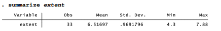
Thus, we show the calculation of summary statistics for a variable named extent as follows:

These typographic conventions exist only in this book, and not within the Stata program itself. Stata can display a variety of onscreen fonts, but it does not use italics in commands. Once Stata log files have been imported into a word processor, or a results table has been copied and pasted, you might want to format them in a Courier font, 10 point or smaller, so that columns will line up correctly.

In its commands and variable names, Stata is case sensitive. Thus, summarize is a command, but Summarize and SUMMARIZE are not. Extent and extent would be two different variables.

2. An Example Stata Session

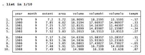
As a preview showing Stata at work, this section retrieves and analyzes a previously-created dataset named Arctic9.dta. This small time series covers satellite-era (1979 to 2011) observations of ice on the Arctic Ocean in September, at the lowest point of its annual cycle. The data come from three different sources (see the appendix on Data Sources). One variable, extent, is a satellite-based measure of the Northern Hemisphere sea area with at least 15% ice concentration each September. Area numbers are somewhat less than extent, representing the area of sea ice itself. Another variable, tempN, describes mean annual surface air temperature above 64°N latitude. Temperatures are expressed as anomalies, which are deviations from the 1951-1980 average, in degrees Celsius. We have 33 observations (years) and 8 variables.

If we might eventually want a record of our session, the best way to prepare for this is by opening a log file at the start. Log files contain commands and results tables, but not graphs. To begin a log file, choose File > Log > Begin … from the top menu bar, and specify a name and folder for the resulting log file. Alternatively, a log file could be started by choosing File > Log > Begin from the top menu bar, or by typing a direct command such as

. log using mondayl

Multiple ways of doing such things are common in Stata. Each way has its own advantages, and each suits different situations or user tastes.

Log files can be created either in a special Stata format (.smcl), or in ordinary text or ASCII format (.log). A .smcl (Stata markup and control language) file will be nicely formatted for viewing or printing within Stata. It could also contain hyperlinks that help to understand commands or error messages. .log (text) files lack such formatting, but are simpler to use if you plan later to insert or edit the output in a word processor. After selecting which type of log file you want, click Save. For this session, we will create a .smcl log file named mondayl.smcl.

An existing Stata-format dataset named Arctic9.dta will be analyzed here. To open or retrieve this dataset, we again have several options:

select File > Open > Arctic9.dta using the top menu bar;

click on  > Arctic9.dta; or

type the command use Arctic9 .

Under its default Windows configuration, Stata looks for data files in the user’s Documents directory. If the file we want is in a different folder, we could specify its location in the use command,

. use C:\books\sws_12\data\Arctic9

or change the session’s default folder by issuing a cd (change directory) command,

. cd C:\books\sws_12\data\

. use Arctic9

or select File > Change Working Directory … from the menus. Often, the simplest way to retrieve a file will be to choose File > Open and browse through folders in the usual way.

To see a brief description of the dataset now in memory, type

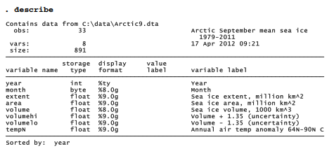
Many Stata commands can be abbreviated to their first few letters. For example, we could shorten describe to just the letter d. Using menus, the same table could be obtained by choosing

Data > Describe data > Describe data in memory > (OK).

This dataset has only 33 observations and 8 variables, so we could list all its contents by typing the command list (or the letter l; or Data > Describe data > List data > (OK)). To save space here we list only the first 10 years, typing list in 1/10:

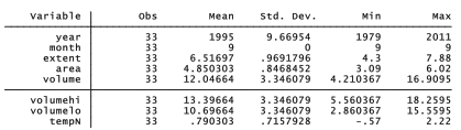
Analysis could begin with a table of means, standard deviations, minimum values, and maximum values. Type summarize or su; or select from the drop-down menus, Statistics > Summaries, tables, and tests > Summary and descriptive statistics > Summary statistics > (OK)

. summarize

To print results from the session so far, click on the Results window and then , or from the menus choose File > Print > Results .

To copy a table, commands, or other information from the Results window into a word processor, drag the mouse to select the results you want, right-click the mouse, and then choose Copy Text from the mouse’s menu. Switch to your word processor and, at the desired insertion point either right-click and Paste or click the word processor’s paste icon. A final step in most cases will be to change the pasted text to a fixed-width font such as Courier.

Arctic sea ice extent, area and volume should be related to annual air temperature, not only because warmer air contributes to ice melting but also because surface air temperatures over ice- free seas will be warmer than temperatures over ice. We can see the correlations among variables by typing correlate followed by a list of variables.

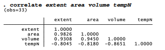
September sea ice extent, area and volume all have strong positive correlations, as one might expect. Their correlation with annual air temperature is negative: the warmer the air, the less ice (or vice versa). The same correlation matrix could be obtained through menus:

Statistics > Summaries, tables, and tests > Summary and descriptive statistics > Correlation and covariance

Then choose the variables to be correlated. Although menu choices often are straightforward to use, you can see that they are more complicated to describe than the simple text commands. From this point on, we will focus primarily on the commands, mentioning menu alternatives only occasionally. Fully exploring the menus, and working out how to use them to accomplish the same tasks, will be left to the reader. For similar reasons, the Stata reference manuals likewise take a command-based approach.

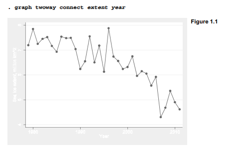
So ice extent, area, volume and temperature all are related. How have they changed over time? Figure 1.1 plots extent against year, produced by the graph twoway connect command. The first-named variable in this command, extent, defines the vertical or y axis; the last-named variable, year, defines the horizontal or x axis. We see an uneven but steepening downward pattern, as September sea ice extent declined by more than a third over this period.

To print this graph, go to the Graph window and click its print icon “ or File > Print. To copy the graph directly into a word processor or other document, right-click on the graph, and select Copy Graph. Switch to your word processor, go to the desired insertion point, and issue an appropriate paste command such as Edit > Paste, Edit > Paste Special (Metafile) , or click a paste icon (different word processors will handle this differently).

To save the graph for future use, either right-click and Save Graph, click in the Graph window, or select File > Save As from the Graph window’s top menu bar. The Save as type submenu offers several different file formats. On a Windows system, the choices include

Stata graph (*.gph) (A “live” graph, containing enough information for Stata to edit)

As-is graph (*.gph) (A more compact Stata graph format)

Windows Metafile (*.wmf)

Enhanced Metafile (*.emf)

Portable Network Graphics (*.png)

TIFF (*.tif)

PostScript (*.ps)

Encapsulated PostScript with or without TIFF preview (*.eps)

Portable Document File (*.pdf)

Other platforms such as Mac or Linux offer different choices for graph file formats. Regardless of which format we want, it often is worthwhile to save one copy of our graph in live .gph format. Such live .gph-format graphs can later be retrieved, combined, recolored or reformatted using the graph use or graph combine commands, or edited using the Graph Editor (Chapter 3).

Through all of the preceding analyses, the log file mondayl.smcl has been storing our results. An easy way to review this file to see what we have done is to open the file in its own Viewer window by selecting

File > Log > View > OK

We could print this log file by clicking the icon on the top bar of the log file’s Viewer window. Log files close automatically at the end of a Stata session, or earlier if instructed by > Close log file, typing the command log close, or by choosing

File > Log > Close

Once closed, the file mondayl.smcl could be opened to view again through File > Log > View or during a subsequent Stata session. To create an output file that can be opened easily by your word processor, either translate the log file from .smcl (a Stata format) to .log (standard ASCII text format) by typing

. translate mondayl.smcl monday1.log

or start out by creating the file in .log instead of .smcl format. You can also start and stop a log file temporarily, any number of times:

File > Log > Suspend

File > Log > Resume

The log icon on Stata’s main icon menu bar can also perform all these tasks.

Source: Hamilton Lawrence C. (2012), Statistics with STATA: Version 12, Cengage Learning; 8th edition.