Competitive Factor Markets

A competitive factor market is one in which there are a large number of sellers and buyers of a factor of production, such as labor or raw mate­rials. Because no single seller or buyer can affect the price of a given factor, each is a price taker. For example, if individual firms that buy lumber to construct homes purchase a small share of the total volume of lumber available, their purchasing decision will have no effect on price. Likewise, if each supplier of lumber controls only a small share of the market, no individual supplier’s decision will affect the price of the lumber that he sells. Instead, the price of lumber (and the total quantity produced) will be determined by the aggregate supply and demand for lumber.

We begin by analyzing the demands for a factor by individual firms. These demands are added to get market demand. We then shift to the supply side of the market and show how market price and input levels are determined.

1. Demand for a Factor Input When Only

One Input Is Variable

Like demand curves for the final goods that result from the production process, demand curves for factors of production are downward sloping. Unlike con- sumers’ demands for goods and services, however, factor demands are derived demands: They depend on, and are derived from, the firm’s level of output and the costs of inputs. For example, the demand of the Microsoft Corporation for computer programmers is a derived demand that depends not only on the current salaries of programmers, but also on how much software Microsoft expects to sell.

To analyze factor demands, we will use the material from Chapter 7 that shows how a firm chooses its production inputs. We will assume that the firm produces its output using two inputs, capital K and labor L, that can be hired at the prices r (the rental cost of capital) and w (the wage rate), respectively.1  We will also assume that the firm has its plant and equipment in place (as in a short- run analysis) and must only decide how much labor to hire.

Suppose that the firm has hired a certain number of workers and wants to know whether it is profitable to hire one additional worker. This will be profit- able if the additional revenue from the output of the worker ’s labor is greater than its cost. The additional revenue from an incremental unit of labor, the marginal revenue product of labor, is denoted MRPL. The cost of an incremen- tal unit of labor is the wage rate, w. Thus, it is profitable to hire more labor if the MRPL is at least as large as the wage rate w.

How do we measure the MRPL? It’s the additional output obtained from the addi-tional unit of this labor, multiplied by the additional revenue from an extra unit of out-put. The additional output is given by the marginal product of labor MPL  and the additional revenue by the marginal revenue MR.

Formally, the marginal revenue product is J)R/J)L, where L is the number of units of labor input and R is revenue. The additional output per unit of labor, the MPL, is given by J)Q/J)L, and marginal revenue, MR, is equal to J)R/J)Q. Because J)R/J)L = (J)R)/(J)Q)(J)Q/J)L), it follows that

MRPL  = (MR)(MPL)                                              (14.1)

This important result holds for any competitive factor market, whether or not the output market is competitive. However, to examine the characteristics of the MRPL, let’s begin with the case of a perfectly competitive output (and input) market. In a competitive output market, a firm will sell all its output at the mar- ket price P. The marginal revenue from the sale of an additional unit of output is then equal to P. In this case, the marginal revenue product of labor is equal to the marginal product of labor times the price of the product:

MRPL  = (MPL)(P)                                                  (14.2)

The higher of the two curves in Figure 14.1 represents the MRPL  curve for a firm in a competitive output market. Note that because there are diminishing marginal returns to labor, the marginal product of labor falls as the amount of labor increases. The marginal revenue product curve thus slopes downward, even though the price of the output is constant.

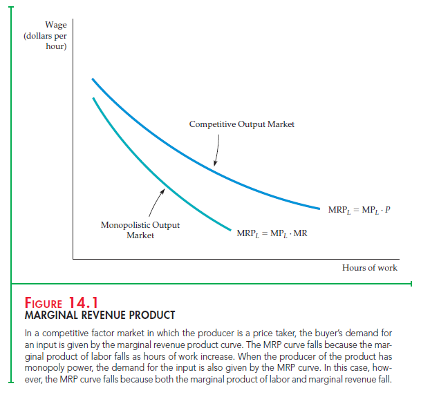
The lower curve in Figure 14.1 is the MRPL  curve when the firm has monop- oly power in the output market. When firms have monopoly power, they face a downward-sloping demand curve and must therefore lower the price of all units of the product in order to sell more of it. As a result, marginal revenue is always less than price (MR < P). This explains why the monopolistic curve lies below the competitive curve and why marginal revenue falls as output increases. Thus the marginal revenue product curve slopes downward in this case because the marginal revenue curve and the marginal product curve slope downward.

Note that the marginal revenue product tells us how much the firm should be willing to pay to hire an additional unit of labor. As long as the MRPL  is greater than the wage rate, the firm should hire more labor. If the marginal revenue prod- uct is less than the wage rate, the firm should lay off workers. Only when the marginal revenue product is equal to the wage rate will the firm have hired the profit-maximizing amount of labor. The profit-maximizing condition is therefore

Figure 14.2 illustrates this condition. The demand for labor curve DL  is the MRPL. Note that the quantity of labor demanded increases as the wage rate falls.

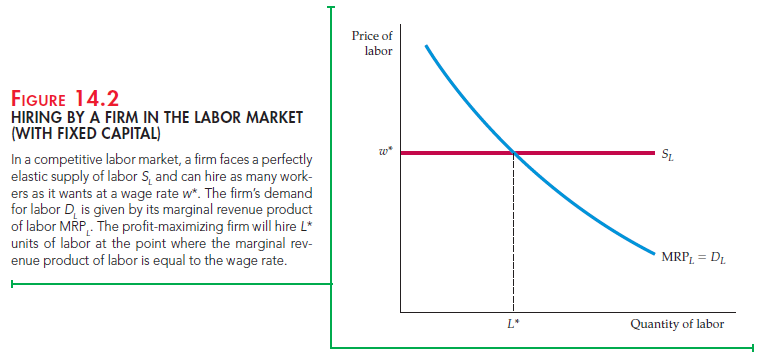
Because the labor market is perfectly competitive, the firm can hire as many workers as it wants at the market wage w* and is not able to affect the market wage. The supply of labor curve facing the firm SL  is thus a horizontal line. The profit-maximizing amount of labor that the firm hires, L*, is at the intersection of the supply and demand curves.

Figure 14.3 shows how the quantity of labor demanded changes in response to a drop in the market wage rate from w1  to w2. The wage rate might decrease if more people entering the labor force are looking for jobs for the first time (as happened, for example, when the baby boomers came of age). The quantity of labor demanded by the firm is initially L1, at the intersection of MRPL  and S1.

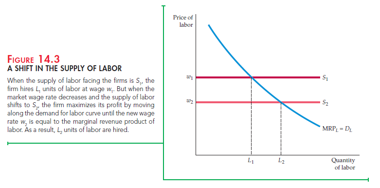
However, when the supply of labor curve shifts from S1  to S2, the wage falls from w1 to w2 and the quantity of labor demanded increases from L1 to L2.

Factor markets are similar to output markets in many ways. For example, the factor market profit-maximizing condition that the marginal revenue product of labor be equal to the wage rate is analogous to the output market condition that marginal revenue be equal to marginal cost. To see why this is true, recall that MRPL = (MPL)(MR) and divide both sides of equation (14.3) by the marginal product of labor. Then,

Because MPL  measures additional output per unit of input, the right-hand side of equation (14.4) measures the marginal cost of an additional unit of out- put (the wage rate multiplied by the labor needed to produce one unit of out- put). Equation (14.4) shows that both the hiring and output choices of the firm follow the same rule: Inputs or outputs are chosen so that marginal revenue (from the sale of output) is equal to marginal cost (from the purchase of inputs). This principle holds in both competitive and noncompetitive markets.

2. Demand for a Factor Input When Several

Inputs Are Variable

When the firm simultaneously chooses quantities of two or more variable inputs, the hiring problem becomes more difficult because a change in the price of one input will change the demand for others. Suppose, for example, that both labor and assembly-line machinery are variable inputs for producing farm equipment. Let’s say that we wish to determine the firm’s demand for labor curve. As the wage rate falls, more labor will be demanded even if the firm’s investment in machinery is unchanged. But as labor becomes less expensive, the marginal cost of producing the farm equipment falls. Consequently, it is profit- able for the firm to increase its output. In that case, the firm is likely to invest in additional machinery to expand production capacity. Expanding the use of machinery causes the marginal revenue product of labor curve to shift to the right; in turn, the quantity of labor demanded increases.

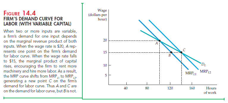
Figure 14.4 illustrates this. Suppose that when the wage rate is $20 per hour, the firm hires 100 worker-hours, as shown by point A on the MRPL1  curve. Now consider what happens when the wage rate falls to $15 per hour. Because the marginal revenue product of labor is now greater than the wage rate, the firm will demand more labor. But the MRPL1  curve describes the demand for labor when the use of machinery is fixed. In fact, a greater amount of labor causes the marginal product of capital to rise, which encourages the firm to rent more machinery as well as hire more labor. Because there is more machinery, the mar- ginal product of labor will increase. (With more machinery, workers can be more productive.) The marginal revenue product curve will therefore shift to the right (to MRPL2). Thus, when the wage rate falls, the firm will use 140 hours of labor. This is shown by a new point on the demand curve, C, rather than 120 hours as given by B. A and C are both on the firm’s demand for labor curve (with machin- ery variable) DL; B is not.

Note that as constructed, the demand for labor curve is more elastic than either of the two marginal product of labor curves (which presume no change in the amount of machinery). Thus, when capital inputs are variable in the long run, there is a greater elasticity of demand because firms can substitute capital for labor in the production process.

3. The Market Demand Curve

When we aggregated the individual demand curves of consumers to obtain the market demand curve for a product, we were concerned with a single industry. However, a factor input such as skilled labor is demanded by firms in many different industries. Moreover, as we move from industry to industry, we are likely to find that firms’ demands for labor (which are derived in part from the demands for the firms’ output) vary substantially. Therefore, to obtain the total market demand for labor curve, we must first determine each industry’s demand for labor, and then add the industry demand curves horizontally. The second step is straightforward. Adding industry demand curves for labor to obtain a market demand curve for labor is just like adding individual product demand curves to obtain the market demand curve for that product. So let’s concentrate our attention on the more difficult first step.

DETERMINING INDUSTRY DEMAND The first step—determining industry demand—takes into account the fact that both the level of output produced by the firm and its product price change as the prices of the inputs to production change. It is easiest to determine market demand when there is a single producer. In that case, the marginal revenue product curve is the industry demand curve for the input. When there are many firms, however, the analysis is more com­plex because of the possible interaction among the firms. Consider, for instance, the demand for labor when output markets are perfectly competitive. Then, the marginal revenue product of labor is the product of the price of the good and the marginal product of labor (see equation 14.2), as shown by the curve MRP_t1 in Figure 14.5 (a).

Suppose initially that the wage rate for labor is $15 per hour and that the firm demands 100 worker-hours of labor. Now the wage rate for this firm falls to $10 per hour. If no other firms could hire workers at the lower wage, then our firm would hire 150 worker-hours of labor (by finding the point on the MRP_t1 curve that corresponds to the $10-per-hour wage rate). But if the wage rate falls for all firms in an industry, the industry as a whole will hire more labor. This will lead to more output from the industry, a shift to the right of the industry supply curve, and a lower market price for its product.

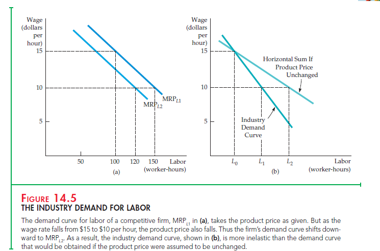
In Figure 14.5 (a), when the product price falls, the original marginal rev­enue product curve shifts downward, from MRP_t1 to MRP_t2. This shift results in a lower quantity of labor demanded by the firm—120 worker-hours rather than 150. Consequently, industry demand for labor will be lower than it would be if only one firm were able to hire workers at the lower wage. Figure (b) illustrates this. The lighter line shows the horizontal sum of the indi­vidual firms’ demands for labor that would result if product price did not change as the wage falls. The darker line shows the industry demand curve for labor, which takes into account the fact that product price will fall as all firms expand their output in response to the lower wage rate. When the wage rate is $15 per hour, industry demand for labor is t₀ worker-hours. When it falls to $10 per hour, industry demand increases to t₁. Note that this is a smaller increase than t₂, which would occur if the product price were fixed. The aggregation of industry demand curves into the market demand curve for labor is the final step: To complete it, we simply add the labor demanded in all industries.

The derivation of the market demand curve for labor (or for any other input) is essentially the same when the output market is noncompetitive. The only difference is that it is more difficult to predict the change in product price in response to a change in the wage rate because each firm in the market is likely to be pricing strategically rather than taking price as given.

Source: Pindyck Robert, Rubinfeld Daniel (2012), Microeconomics, Pearson, 8th edition.